Time Series Comparison

This tutorial covers the comparison between time series signals and the calculation of metrics. Starting from simple subtraction, metrics like root mean squared error for upper and lower boundaries (envelope) are calculated. Finally, step response data is analyzed. The tutorial also illustrates some helper functions for plotting (e.g. fill between two time series).

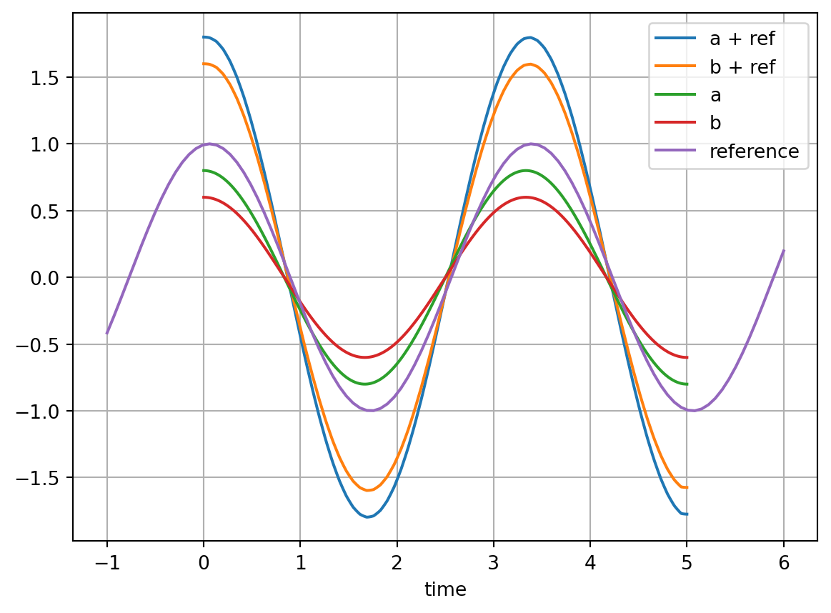
1 Addition and Subtraction

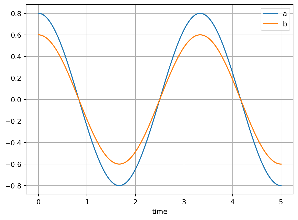
First we create a time series with two curves between 0 and 5 seconds. The time samples are randomly varied (sample time is not constant). This could be for example results of simulations with an adaptive (variable) step solver. Note that there is a separate tutorial on signal generation.

import numpy as np
import pandas as pd
from matplotlib import pyplot as plt

from trimes.signal_generation import PeriodicSignal

t_start = 0
t_end = 5
average_sample_time = 1e-3
time = np.arange(t_start, t_end, average_sample_time)
time = time + (np.random.rand(len(time)) - 0.5) * 1e-5

sig_a = PeriodicSignal(time, mag=0.8, f=0.3)
sig_b = PeriodicSignal(time, mag=0.6, f=0.3)

df_ts = pd.DataFrame({"a": sig_a.get_signal(), "b": sig_b.get_signal()}, index=time)
df_ts.index.name = "time"
df_ts.plot(grid=True)

Next we create a reference signal with a different sampling time compared to above.

time = np.linspace(t_start - 1, t_end + 1, 100)
sig_ref = PeriodicSignal(time, mag=1, f=0.3, phi=-2)
series_reference = sig_ref.get_signal_series()

df_ts.plot()
series_reference.name = "reference"
series_reference.plot(grid=True)

plt.legend(loc="upper center")

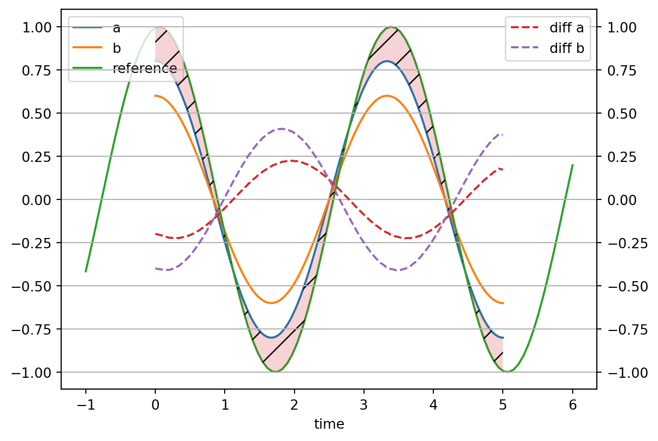
We calculate the difference between signals ‘a’/‘b’ and the reference. The reference is automatically resampled according to the sample time of signals ‘a’/‘b’, i.e. the option resample_reference is set to True. The option is available in most of the functions in the following but is set to False by default to avoid unnecessary resampling that deteriorates the performance. There is also the option resample_ts to resample the time series ‘a’/‘b’ to the reference time base. Instead of resampling at every function call, consider using resample from trimes.base to align the sample time only once before the comparison if the sample time remains constant.

A diagram with two y-axes is used for visualization (original signals on the left axis, difference on the right). In addition, the area between ‘b’ and ‘reference’ is filled.

from trimes.comparison import subtract
from trimes.plots import plot_2y, fill_between

difference = subtract(df_ts, series_reference, resample_reference=True)
difference.columns = ("diff a", "diff b")

signals_a_b_and_reference = pd.concat([df_ts, series_reference])
ax1, ax2 = plot_2y(
    signals_a_b_and_reference, difference, kwargs_ax2={"linestyle": "--"}
)
fill_between(df_ts["a"], series_reference, alpha=0.2, hatch="/")
plt.grid()

Addition works similar:

from trimes.comparison import add

sum = add(df_ts, series_reference, resample_reference=True)
sum.columns = ("a + ref", "b + ref")
ax = sum.plot()
signals_a_b_and_reference.plot(ax=ax)
plt.grid()

2 Compare to Reference Signal

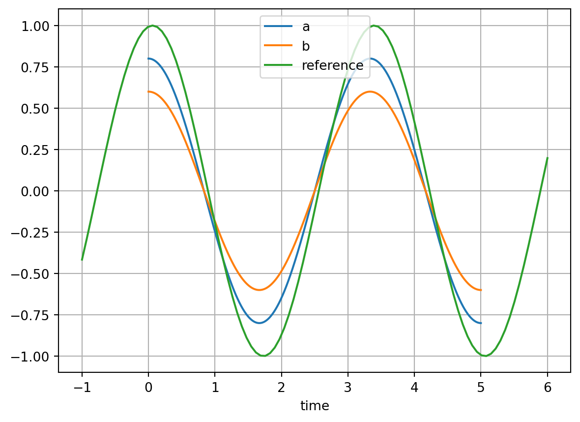
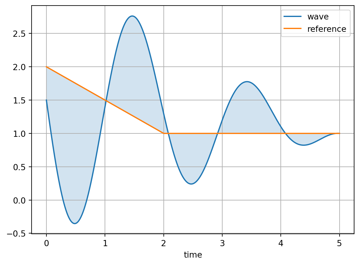
A common use case is to check how well a signal aligns with a reference signal. We first create a periodic signal and a reference (note that there is a separate tutorial on signal generation).

from trimes.signal_generation import PeriodicSignal, linear_time_series
from trimes.plots import fill_between

sample_time = 1e-3
signal = PeriodicSignal(
    np.arange(0, 5 + sample_time, sample_time),
    f=0.5,
    offset=(1.5, 1),
    mag=(2, 0.01),
    phi=np.pi / 2,
)
wave = signal.get_signal_series()
wave.name = "wave"
ax = wave.plot()

t = (0, 2, 5)
y = (2, 1, 1)
sample_time = 1e-3
reference = linear_time_series(t, y, sample_time)
reference.name = "reference"
reference.plot(ax=ax, grid=True)
fill_between(wave, reference, alpha=0.2)
plt.legend()

comparison_series and comparison_df calculate any error metric (default is integral_abs_error, i.e. area) for series and dataframes. Some metrics are defined in trimes.metrics. Further metrics from the scikit-learn package can be used.

from trimes.comparison import comparison_series, comparison_df
from trimes.metrics import integral_squared_error
from sklearn.metrics import root_mean_squared_error

print(comparison_series(wave, reference))
print(comparison_series(wave, reference, metric=integral_squared_error))

df_waves = pd.concat([wave, wave * 0.1], axis=1)
print(
    comparison_df(
        df_waves, reference, metric=root_mean_squared_error, sample_time=sample_time
    )
)

3.4983548161487557
0.004193576094696082
[0.91582761 1.13841978]

3 Boundaries and Envelopes

3.1 Create Boundaries as Linear Time Series Signals

We will create boundaries and check whether a time series signal remains within the envelope and calculate error metrics.

from trimes.signal_generation import linear_time_series, mirror_y

t = (0, 2, 3, 3, 5)
y = (2, 2, 1.5, 1.2, 1.2)
sample_time = 1e-3
ts = linear_time_series(t, y, sample_time)
ts_envelope = mirror_y(ts, 1, inplace=True)
ts_envelope.columns = ("upper boundary", "lower boundary")
ts_envelope.plot(grid=True, linestyle="--")

Create the periodic signal:

from trimes.signal_generation import PeriodicSignal

signal = PeriodicSignal(
    np.arange(0, 5 + sample_time, sample_time),
    f=0.5,
    offset=(1.5, 1),
    mag=(2, 0.01),
    phi=np.pi / 2,
)
wave = signal.get_signal_series()
wave.name = "wave"
ax = plt.subplot()
wave.plot(ax=ax)
ts_envelope.plot(ax=ax, linestyle="--")
plt.legend()
plt.grid()

3.2 Check Boundaries

greater_than_series and smaller_than_series compare the wave to the boundary and return a boolean array.

from trimes.comparison import greater_than_series

upper_boundary = ts_envelope.iloc[:, 0]
greater_than_series(wave, upper_boundary)

array([False, False, False, ..., False, False, False])

apply_operator_series can be used in a similar way using any suitable operator from the built-in operator module.

import operator
from trimes.comparison import apply_operator_series
from trimes.plots import fill_between

greater = apply_operator_series(wave, ts_envelope.iloc[:, 0], operator.gt)
smaller = apply_operator_series(wave, ts_envelope.iloc[:, 1], operator.lt)

ax = plt.subplot()
wave.plot(ax=ax)

ts_envelope.plot(ax=ax, linestyle="--")
fill_between(wave.iloc[greater], ts_envelope.iloc[greater, 0], alpha=0.5)
fill_between(wave.iloc[smaller], ts_envelope.iloc[smaller, 1], alpha=0.5)
plt.legend()
plt.grid()

For convenience there is also a method that checks upper and lower boundary at once:

from trimes.comparison import outside_envelope

outside_envelope(wave, ts_envelope)

array([False, False, False, ..., False, False, False])

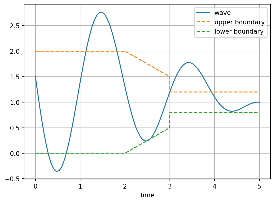
If you are interested in the time a condition is fullfilled (like a signal being outside an envelope), the get_time_bool function calculates the duration from a boolean array and the sampling time.

from trimes.comparison import get_time_bool

out = outside_envelope(wave, ts_envelope)
get_time_bool(out, ts_envelope.index.values)

np.float64(2.1029999999999998)

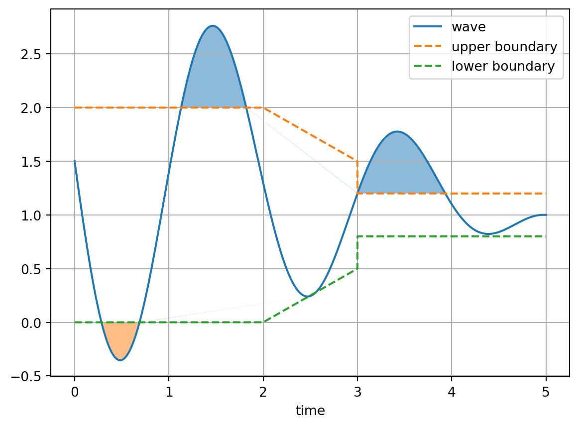
3.3 Calculate Metric

Next we calculate metrics such as the area where the wave exceeds the envelope. comparison_series/comparison_df accept an operator as input argument to consider only time spans where the condition is True.

from trimes.comparison import comparison_series, comparison_df
from trimes.metrics import integral_squared_error
from sklearn.metrics import root_mean_squared_error

print(
    comparison_series(
        wave,
        ts_envelope.iloc[:, 0],
        operator.gt,
    )
)
print(
    comparison_series(
        wave, ts_envelope.iloc[:, 1], operator.lt, metric=root_mean_squared_error
    )
)
df_waves = pd.concat([wave, wave * 1.1], axis=1)
print(
    comparison_df(
        df_waves,
        ts_envelope.iloc[:, 0],
        operator.gt,
        metric=integral_squared_error,
    )
)

0.6832649919854159
0.07301156189253198
[0.00036104 0.00072028]

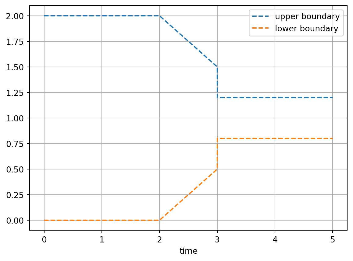
For convenience there are also methods for envelopes instead of a single boundary.

from trimes.comparison import envelope_comparison_series, envelope_comparison_df

envelope_comparison_series(wave, ts_envelope)
envelope_comparison_df(df_waves, ts_envelope)

array([0.77815754, 1.11895373])

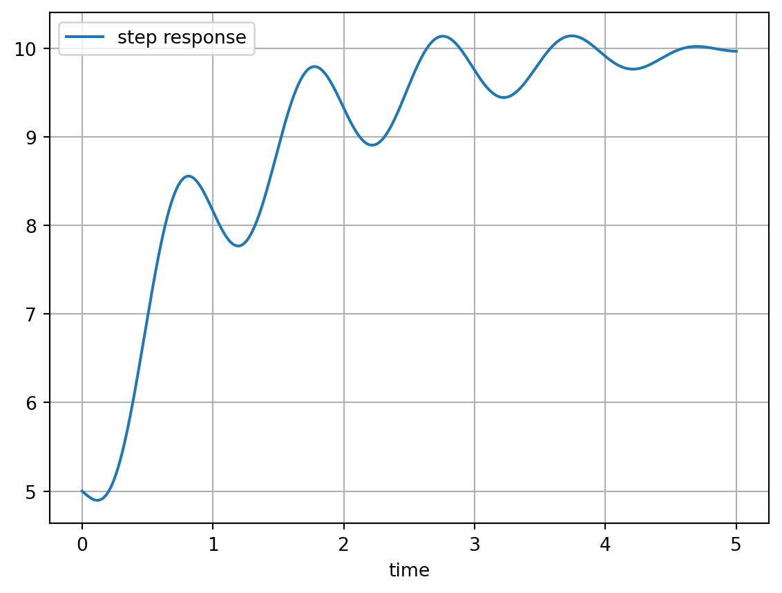
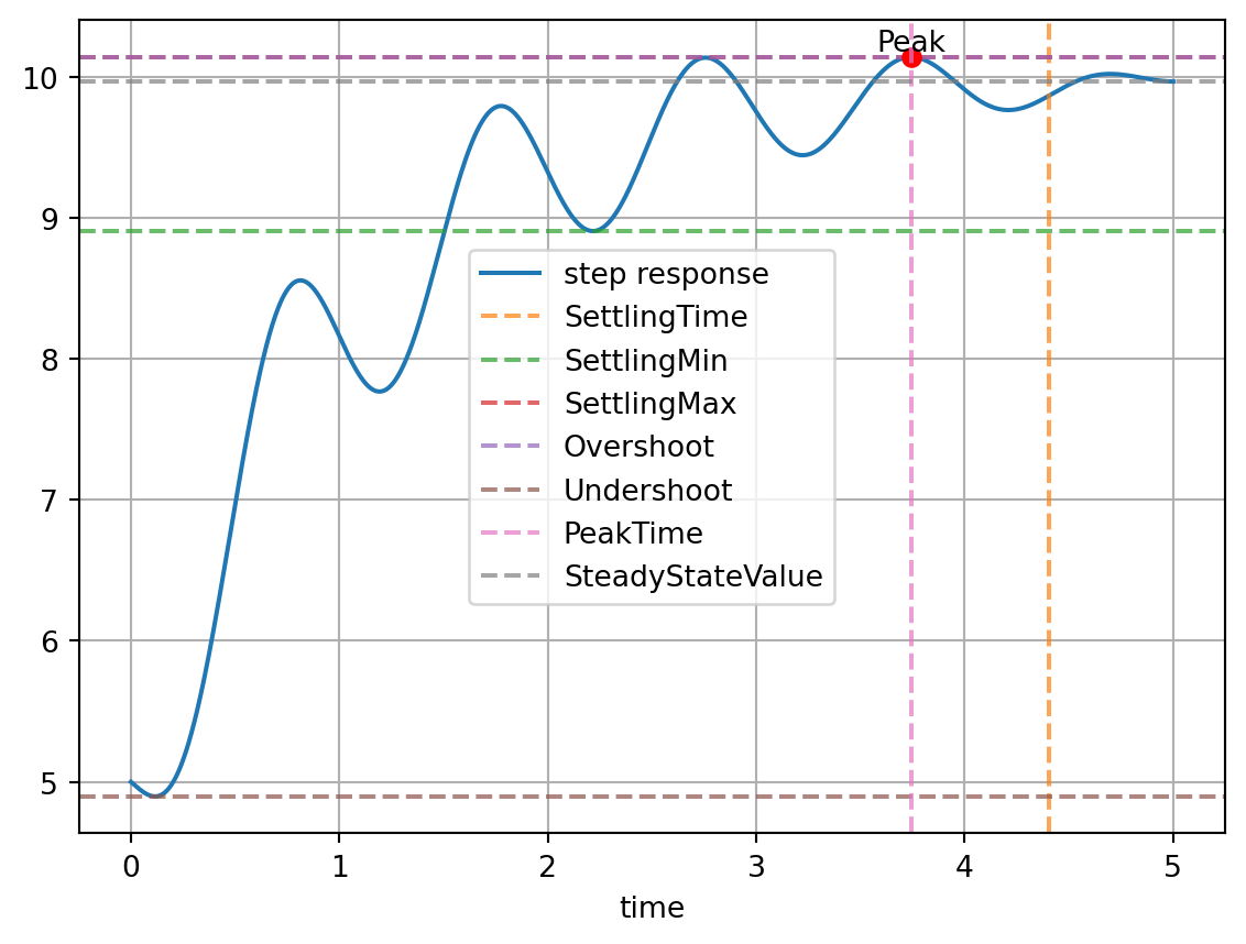
4 Step Response Info

trimes provides an interface to the control package to get the step response info (overshoot etc.) of time series. Let’s first create a step response signal.

t = np.arange(0, 5 + sample_time, sample_time)
offset = 10 - 5 * np.exp(-t)
step_response = PeriodicSignal(
    np.arange(0, 5 + sample_time, sample_time),
    f=1,
    offset=offset,
    mag=(1, 0.01),
    phi=np.pi / 2,
)
step_series = step_response.get_signal_series()
step_series.name = "step response"
step_series.plot(grid=True)
plt.legend()

Get the step response info. Note that the y-values in the results are relative to the initial value.

from trimes.control import step_info_series

info = step_info_series(step_series)
info

{'RiseTime': np.float64(1.303),
 'SettlingTime': np.float64(4.405),
 'SettlingMin': np.float64(3.906303780009649),
 'SettlingMax': np.float64(5.140223553657352),
 'Overshoot': np.float64(3.501861127732394),
 'Undershoot': np.float64(2.0758071455346307),
 'Peak': np.float64(5.140223553657352),
 'PeakTime': np.float64(3.742),
 'SteadyStateValue': np.float64(4.966310265004573)}

There is also a function to illustrate the results.

from trimes.control import plot_step_info

step_series.plot(grid=True)
plot_step_info(step_series, info)
plt.legend()

4.896908976649615