import numpy as np
from matplotlib import pyplot as pltTime Series Generation
This tutorial covers the generation of time series signals. It is shown how to create linear interpolated signals and periodic signals (superimposing several frequencies).
1 Linear Signals
Linear interpolated time series signals can be created by specifying points in time t and the corresponding values y:
from trimes.signal_generation import linear_time_series

t = (0, 2, 2, 3, 5)
y = (2, 2, 1.5, 1.2, 1.2)
sample_time = 1e-3

ts = linear_time_series(t, y, sample_time)
ts.plot(grid=True)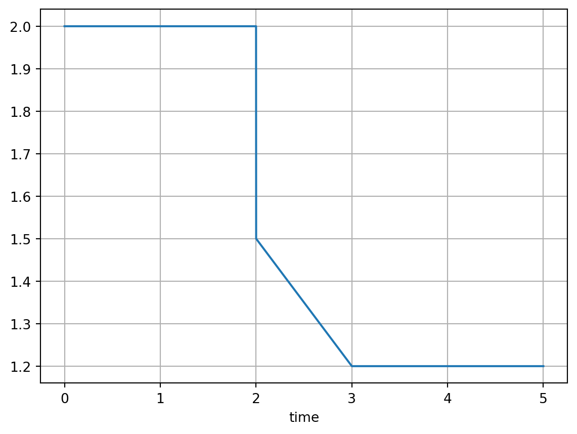
If y is a list, several lines are generated:
t = (0, 2, 2, 3, 5)
y = [(2, 2, 1.5, 1.2, 1.2), (0, 1, 1, 1, 1)]

ts = linear_time_series(t, y, sample_time)
ts.columns = ("upper boundary", "lower boundary")
ts.plot(grid=True)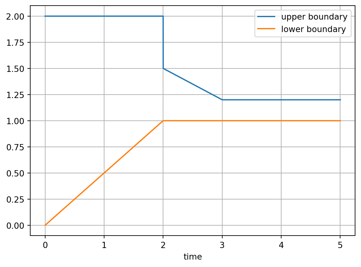
Symmetric signals can also be created using mirror_y (mirroring of the signal at a y-value):
from trimes.signal_generation import mirror_y

upper_boundary = ts.iloc[:, 0]
ts_envelope = mirror_y(upper_boundary, 1, inplace=True)
ts_envelope.columns = ("upper boundary", "lower boundary")
ts_envelope.plot(grid=True)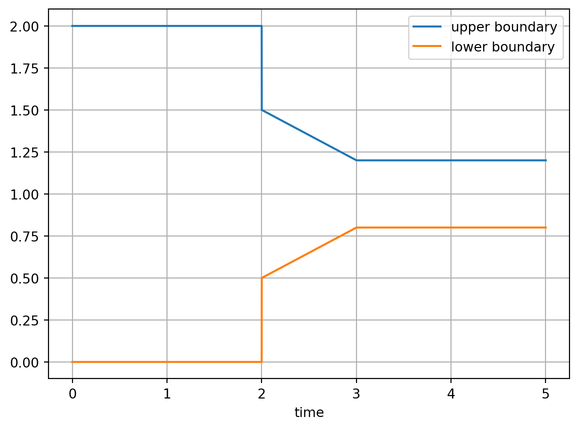
2 Discrete Linear Signals
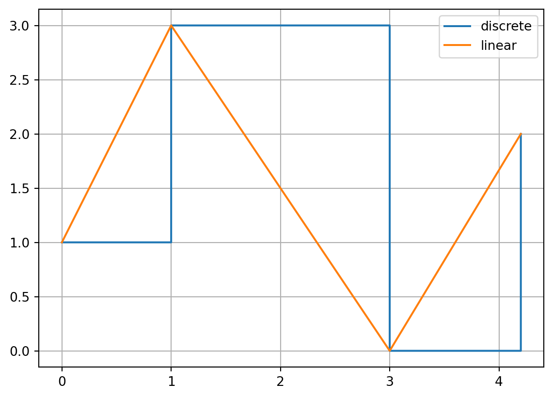
In the above examples, we created discrete steps from one time step to the other (discontinuity) by setting two consecutive time steps with the same value (e.g. t = (0, 2, 2, 3, 5)). If you want to create a signal solely containing discrete steps and don’t want to type the values of each step twice, there is a convenience function which accepts a Timeseries as input:
from trimes.signal_generation import discretize
import pandas as pd

df = pd.DataFrame((1, 3, 0, 2))
df.index = (0, 1, 3, 4.2)
df.columns = ["linear"]

ts = discretize(df.copy())
ts.columns = ["discrete"]
ax = ts.plot()
df.plot(ax=ax, grid=True)

ts| discrete | |
|---|---|
| 0.000000 | 1 |
| 0.999999 | 1 |
| 1.000000 | 3 |
| 2.999999 | 3 |
| 3.000000 | 0 |
| 4.199999 | 0 |
| 4.200000 | 2 |
3 Periodic Signals
The PeriodicSignal class can be used to create periodic signals of any shape (flexibly set parameters like frequency, magnitude, offset and initial angle). By default, cosine signals are created:
from trimes.signal_generation import PeriodicSignal

sample_time = 1e-4
mag = 110 * np.sqrt(2) / np.sqrt(3)
t = np.arange(0, 0.1, sample_time)
cosine_wave = PeriodicSignal(t, f=50, mag=mag, offset=10, phi=np.pi * 0.3)
cosine_wave_series = cosine_wave.get_signal_series()
cosine_wave_series.plot()
plt.grid()
plt.show()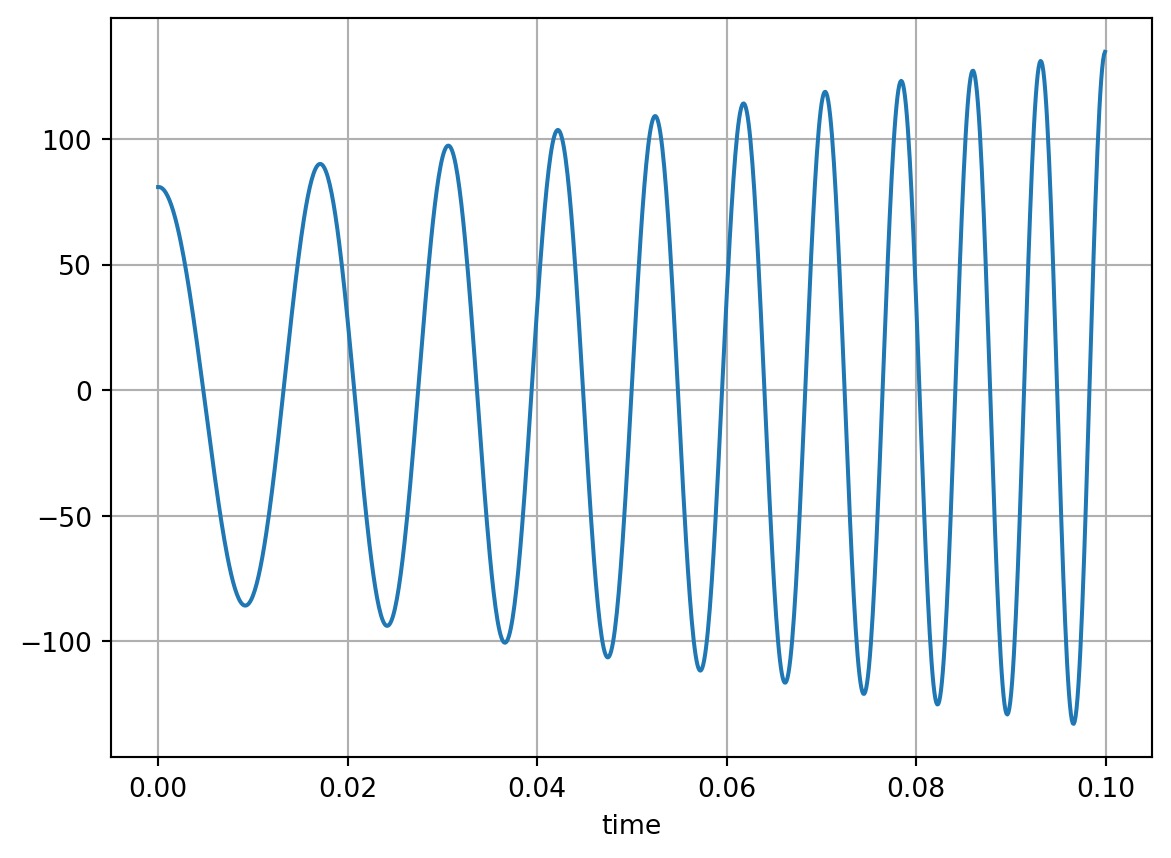
To create gradients, use tuples as parameters (don’t use lists).
plt.close("all")

cosine_wave = PeriodicSignal(
    np.arange(0, 0.1, sample_time), f=(50, 150), mag=(0.9 * mag, 1.5 * mag)
)
cosine_wave.plot(grid=True)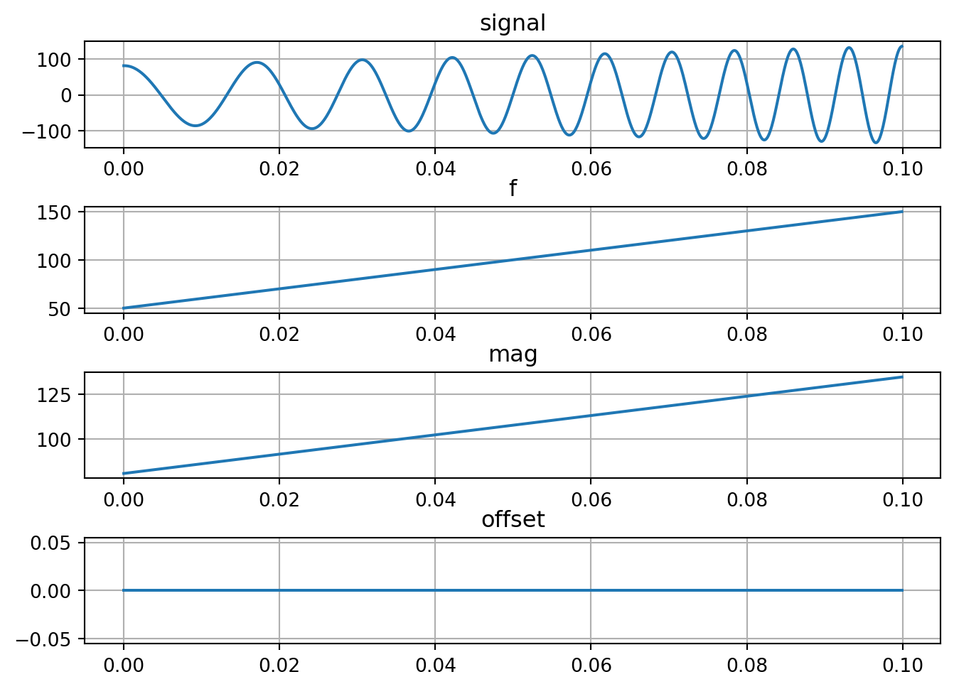
The plot_with_attributes illustrates the signal as well as its parameters over time.
cosine_wave.plot_with_attributes()
plt.grid()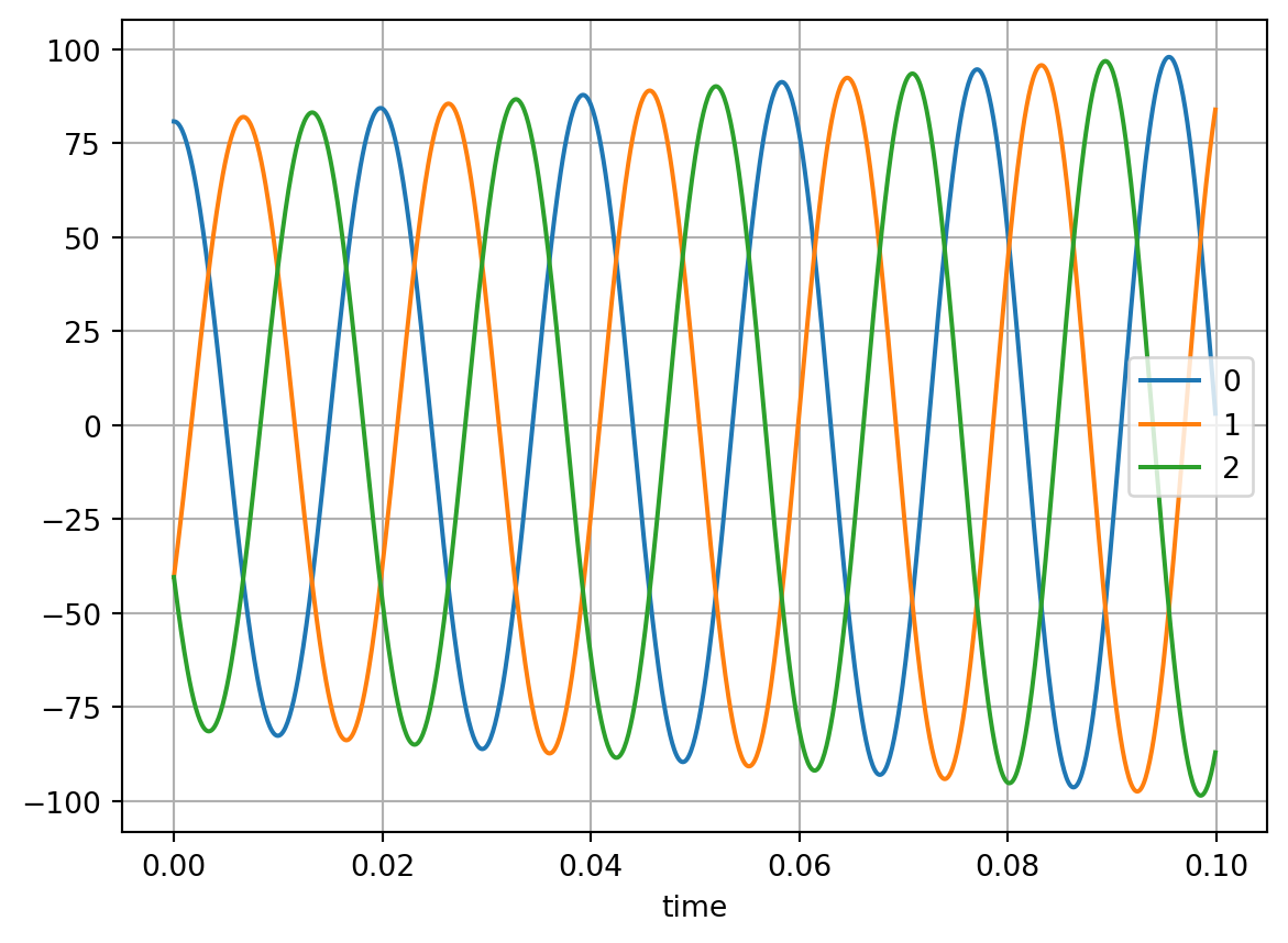
Symmetric multi-phase signals can be created based on the PeriodicSignal class by using get_signal_n_phases (angular phase difference between signals is \(360/n\)):
cosine_wave = PeriodicSignal(
    np.arange(0, 0.1, sample_time), f=(50, 55), mag=(0.9 * mag, 1.1 * mag)
)
cosine_wave_series_3_phase = cosine_wave.get_signal_n_phases(3)
cosine_wave_series_3_phase.plot(grid=True)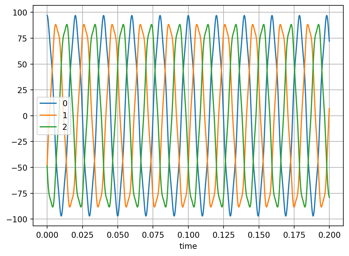
Signals can be superimposed and concatenated by creating an array of signals. The rows of the array are superimposed and the resulting column is concatenated. The following signal is created: - two time periods (with varying frequencies) - 0-0.1 s - 0.1-0.2 s - several frequencies are superimposed: - fundamental: \(50\) Hz (actually varies between \(50\) and \(60\) Hz) - fifth harmonic: \(5*50=250\) Hz - negative sequence: rotating with \(-50\) Hz (actually varies between \(-50\) and \(-60\) Hz) - \(3\) phases
from trimes.signal_generation import (
    superimpose_and_concat_periodic_signals,
)

time_spans = [np.arange(0, 0.1, sample_time), np.arange(0.1, 0.2, sample_time)]
signals = [
    [
        PeriodicSignal(time_spans[0], f=(50, 60), mag=mag),
        PeriodicSignal(time_spans[0], f=(50 * 5, 60 * 5), mag=0.05 * mag),
        PeriodicSignal(time_spans[0], f=(-50, -60), mag=0.03 * mag),
    ],
    [
        PeriodicSignal(time_spans[1], f=50, mag=mag),
        PeriodicSignal(time_spans[1], f=5 * 50, mag=0.05 * mag),
        PeriodicSignal(time_spans[1], f=-50, mag=0.03 * mag),
    ],
]
res = superimpose_and_concat_periodic_signals(
    signals, num_phases=3,
)
res.plot()
plt.grid()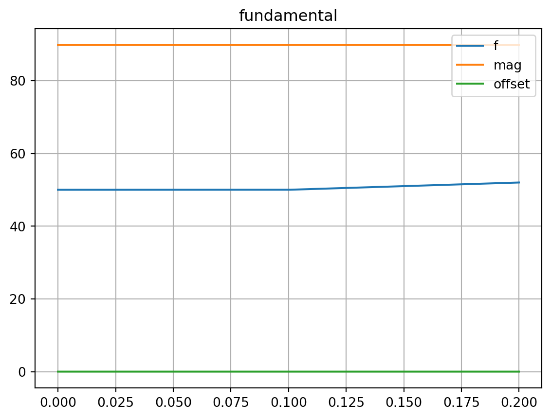
Notice that the signals are continuous at the transition between periods (at t = 0.1 s), since the final angle of the previous period is automatically carried over as the initial angle of the next. This behavior can be disabled, in which case the initial angle resets to zero at each period boundary, resulting in a discontinuity at t = 0.1 s:
res = superimpose_and_concat_periodic_signals(
    signals, num_phases=3, angle_continuation=False
)
res.loc[0.08:0.12, :].plot()
plt.grid()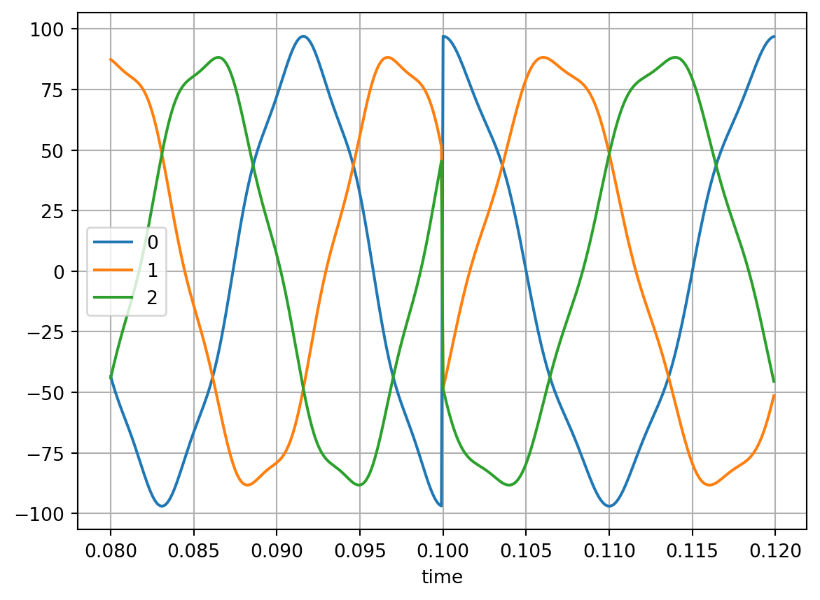
It is also possible to specify a certain angular jump at the transition:
res = superimpose_and_concat_periodic_signals(
    signals, num_phases=3, angular_jump=[np.pi/2] # 90 degree angular jump
)
res.loc[0.08:0.12, :].plot()
plt.grid()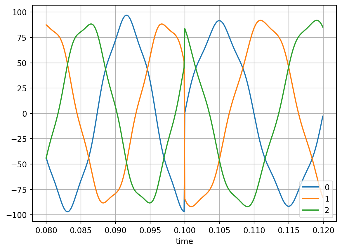
The parameters of the signals can be exctracted using get_attributes_of_superimposed_and_concatenated_signals_over_time and illustrated:
from trimes.signal_generation import (
get_attributes_of_superimposed_and_concatenated_signals_over_time,
)
attrs_of_columns = get_attributes_of_superimposed_and_concatenated_signals_over_time(
signals
)
attrs_of_columns[0].plot(title="fundamental")
plt.grid()
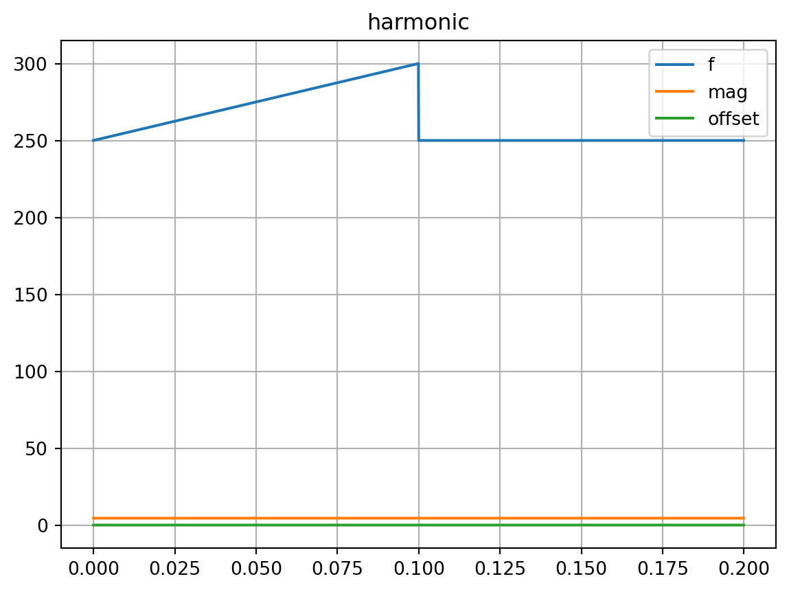
attrs_of_columns[1].plot(title="harmonic")
plt.grid()
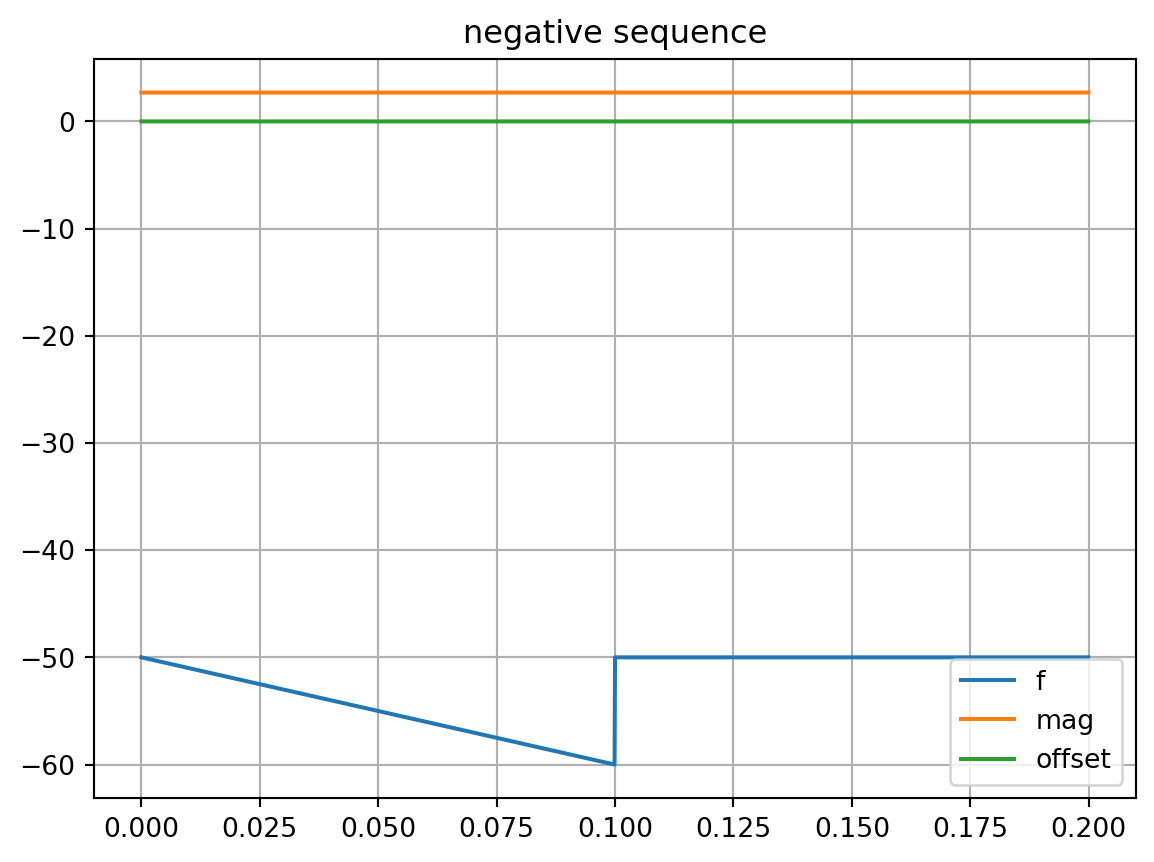
attrs_of_columns[2].plot(title="negative sequence")
plt.grid()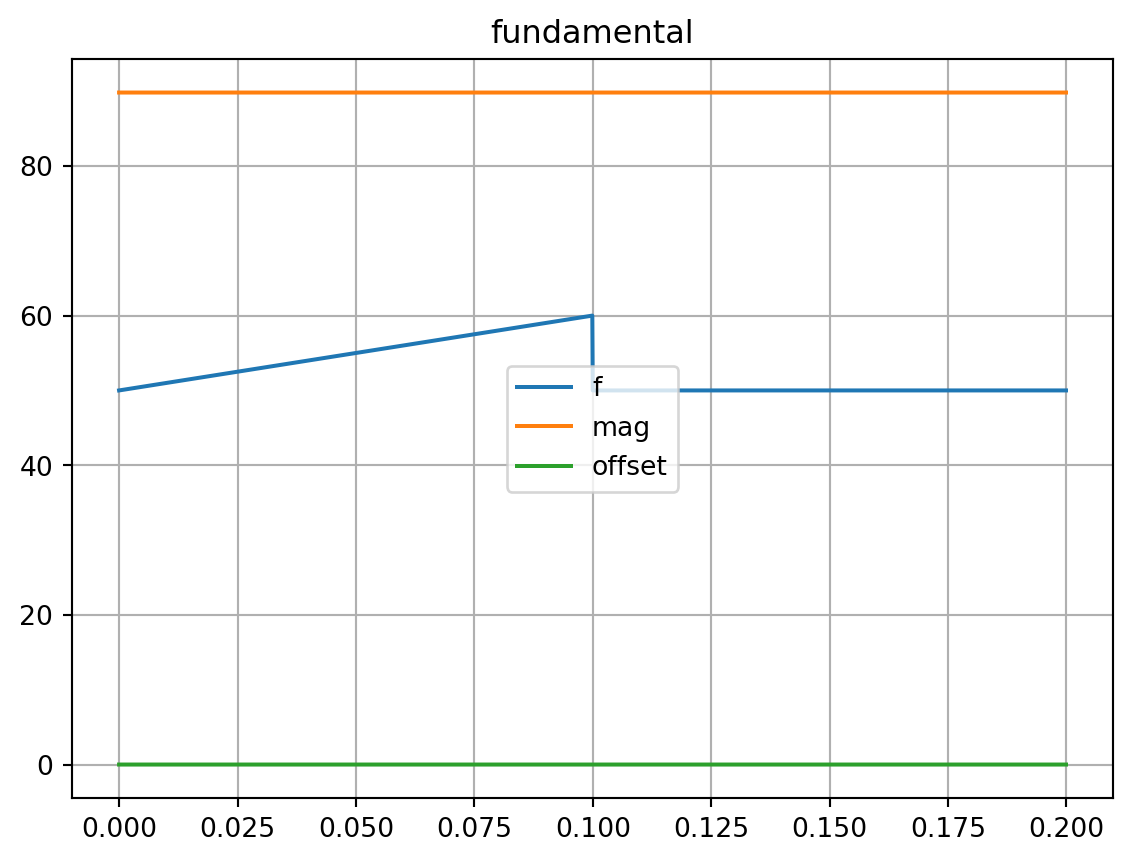
4 Noise
To illustrate the addition of noise to signals, we first create a “clean” periodic three-phase signal.
import numpy as np
import pandas as pd

sample_time = 1e-4
mag = 110 * np.sqrt(2) / np.sqrt(3)
t = np.arange(0, 0.1, sample_time)
cosine_wave = PeriodicSignal(t, f=50, mag=mag, offset=10, phi=np.pi * 0.3)
cosine_wave_series = cosine_wave.get_signal_n_phases(3)
cosine_wave_series.plot()
plt.grid()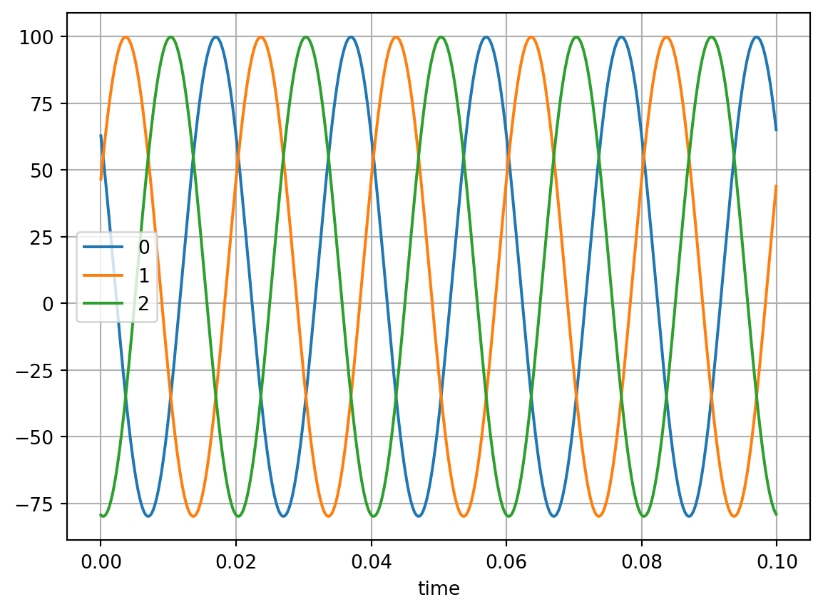
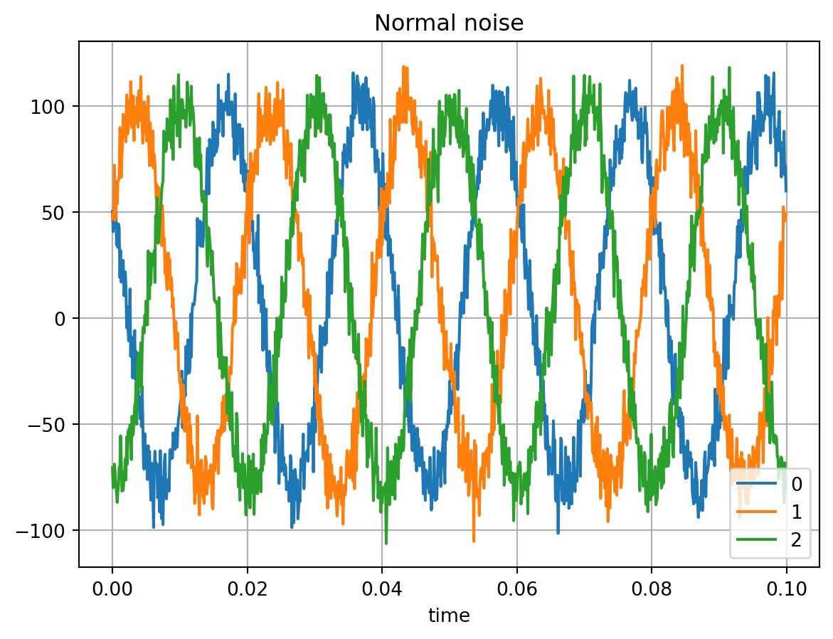
There are functions to add normal and uniform distributed noise to time series.
from trimes.signal_generation import add_normal_noise, add_uniform_noise
cosine_normal_noise = add_normal_noise(cosine_wave_series, 0.1*mag)
cosine_normal_noise.plot()
plt.grid()
plt.title("Normal noise")
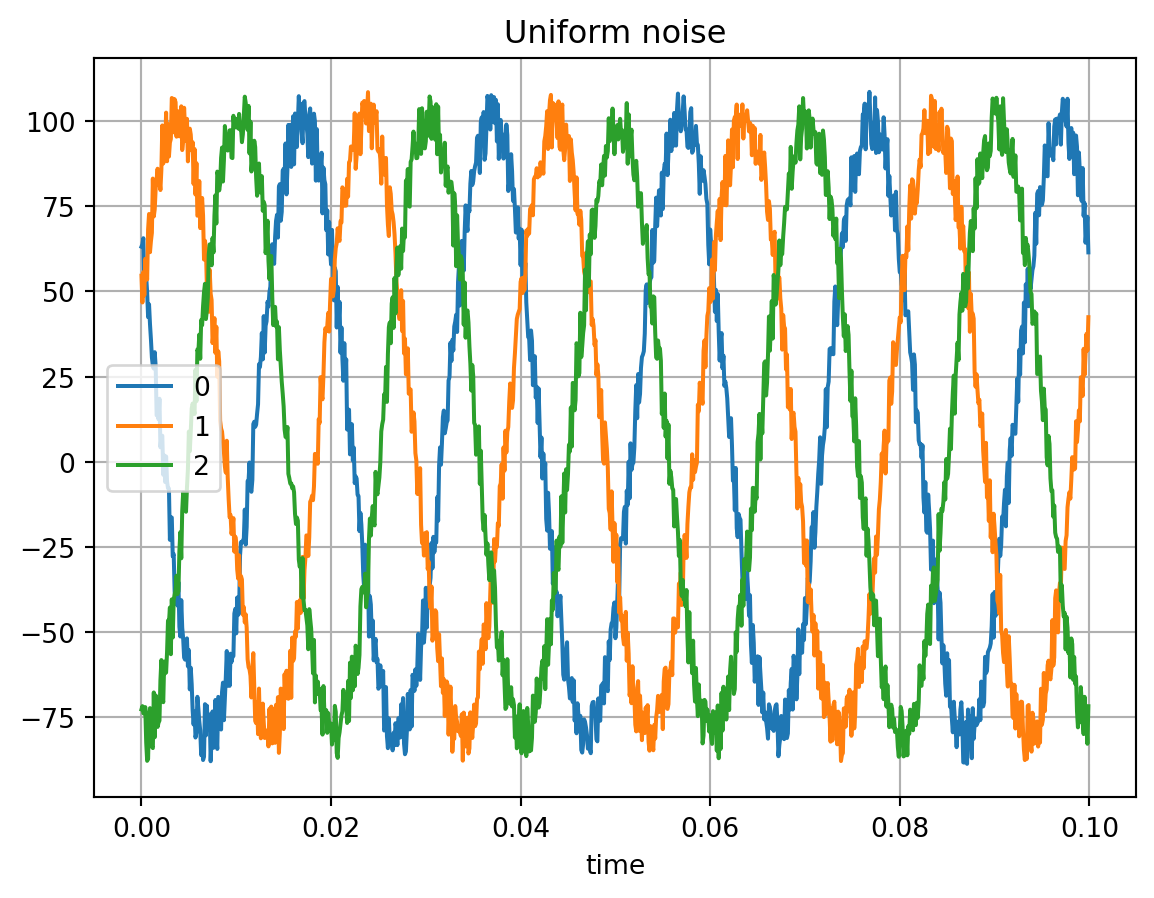
cosine_normal_noise = add_uniform_noise(cosine_wave_series, -0.1*mag, 0.1*mag)
cosine_normal_noise.plot()
plt.grid()
plt.title("Uniform noise")Text(0.5, 1.0, 'Uniform noise')