This tutorial demonstrates several signal processing methods, including:
Moving average (rolling mean)
Filtering (e.g., PT1)
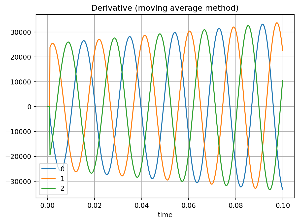
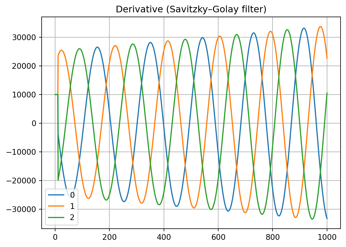
Derivatives
Fourier analysis
Root mean square (RMS)
Please note that the current functionality is limited and will be extended in future versions.
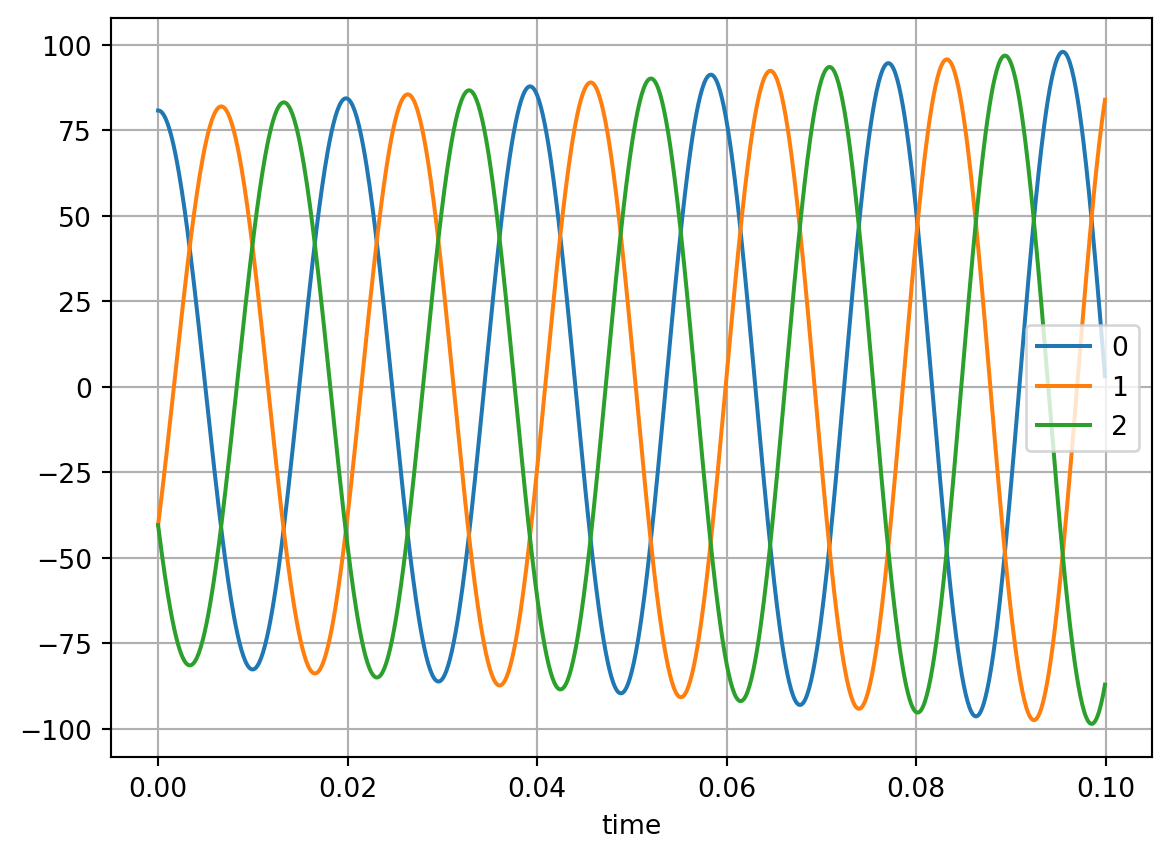
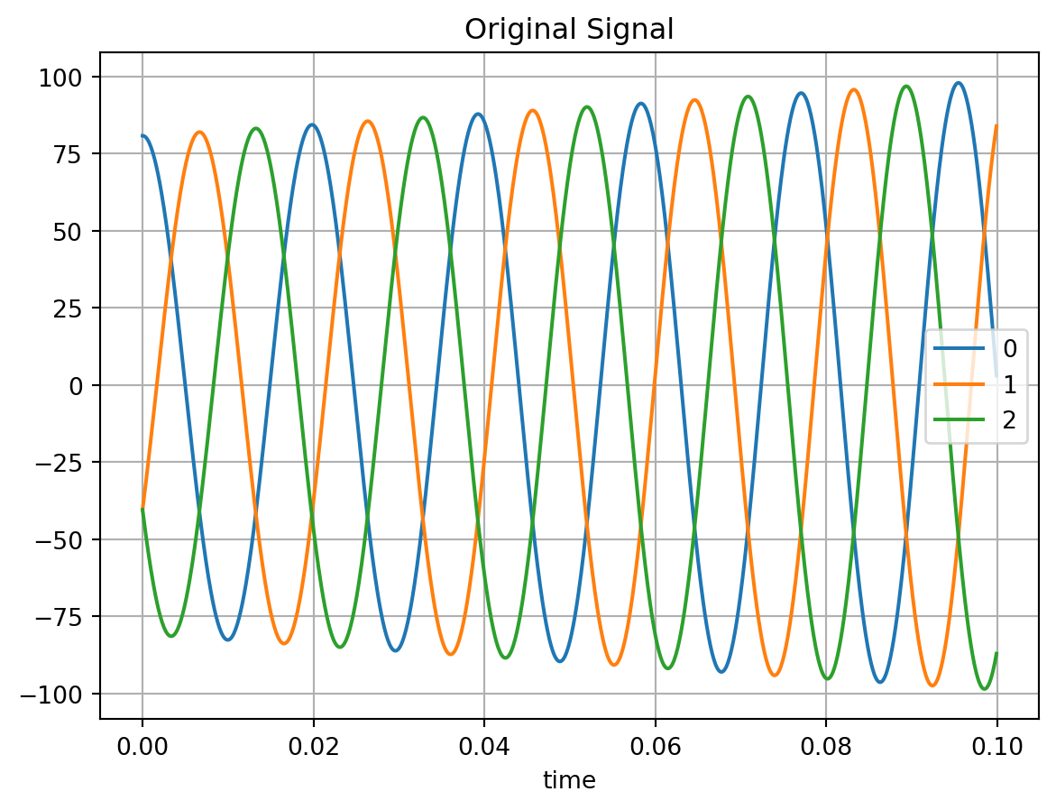
We begin by generating a test signal to which the processing methods will be applied. A three-phase signal with varying frequency and amplitude is used.
Padding is a key concept in many signal processing algorithms. For example, when computing a moving average, valid results are only available after a number of samples equal to the window length. However, it is often desirable that the output signal has the same length as the input signal.
The question then becomes how to fill the undefined boundary values. By default, trimes pads with zeros at the beginning. Internally, it uses numpy.pad, so custom padding behavior can be specified via corresponding keyword arguments.
The number of samples per averaging window (e.g., one period at 50 Hz) can be computed as:
samples_per_window =int(1/ (sample_time *50))
Two padding examples—padding only at the start and padding at both the start and end (each with length 0.5 * samples_per_window) are shown in Section Section 2. For further details, refer to the NumPy documentation for numpy.pad (numpy.org/doc/stable/reference/generated/numpy.pad.html).
2 Moving Average (Rolling Mean)
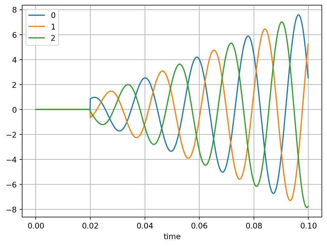
We compute the moving average over one period (assuming 50 Hz) using the default padding (zeros added at the beginning).
from trimes.signal_processing import average_rollingavg = average_rolling( cosine_wave_series_3_phase, samples_per_window=samples_per_window)avg.plot()
The moving average increases slightly due to the frequency gradient in the signal and its deviation from 50 Hz.
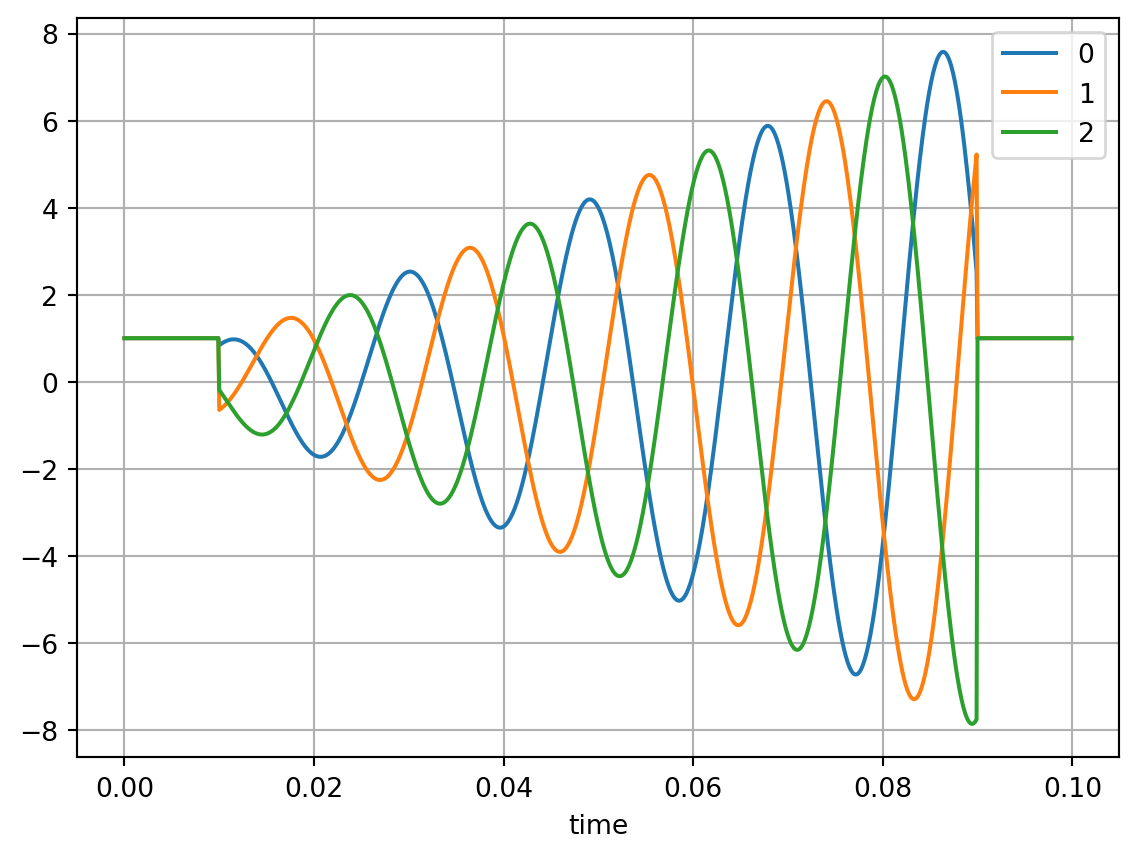
Next, we illustrate custom padding by adding ones at both the beginning and the end.
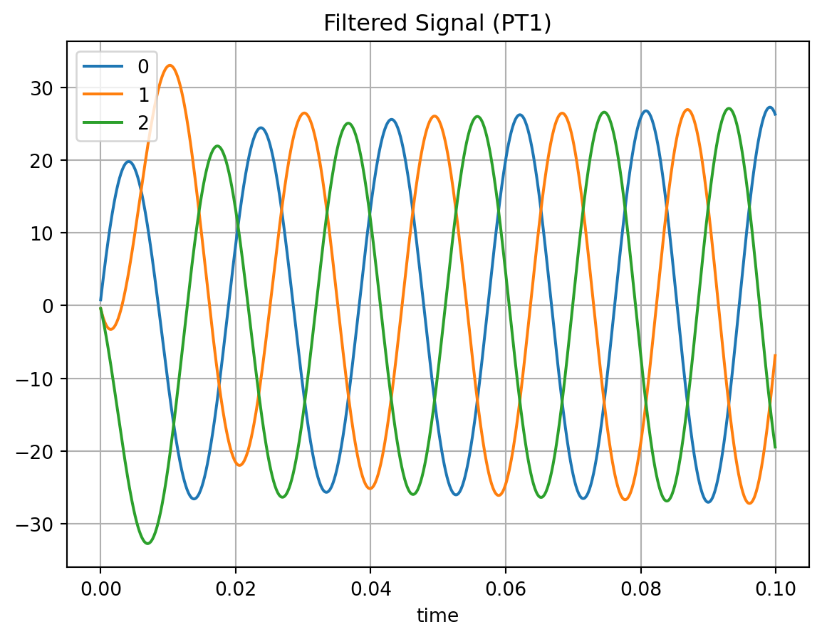
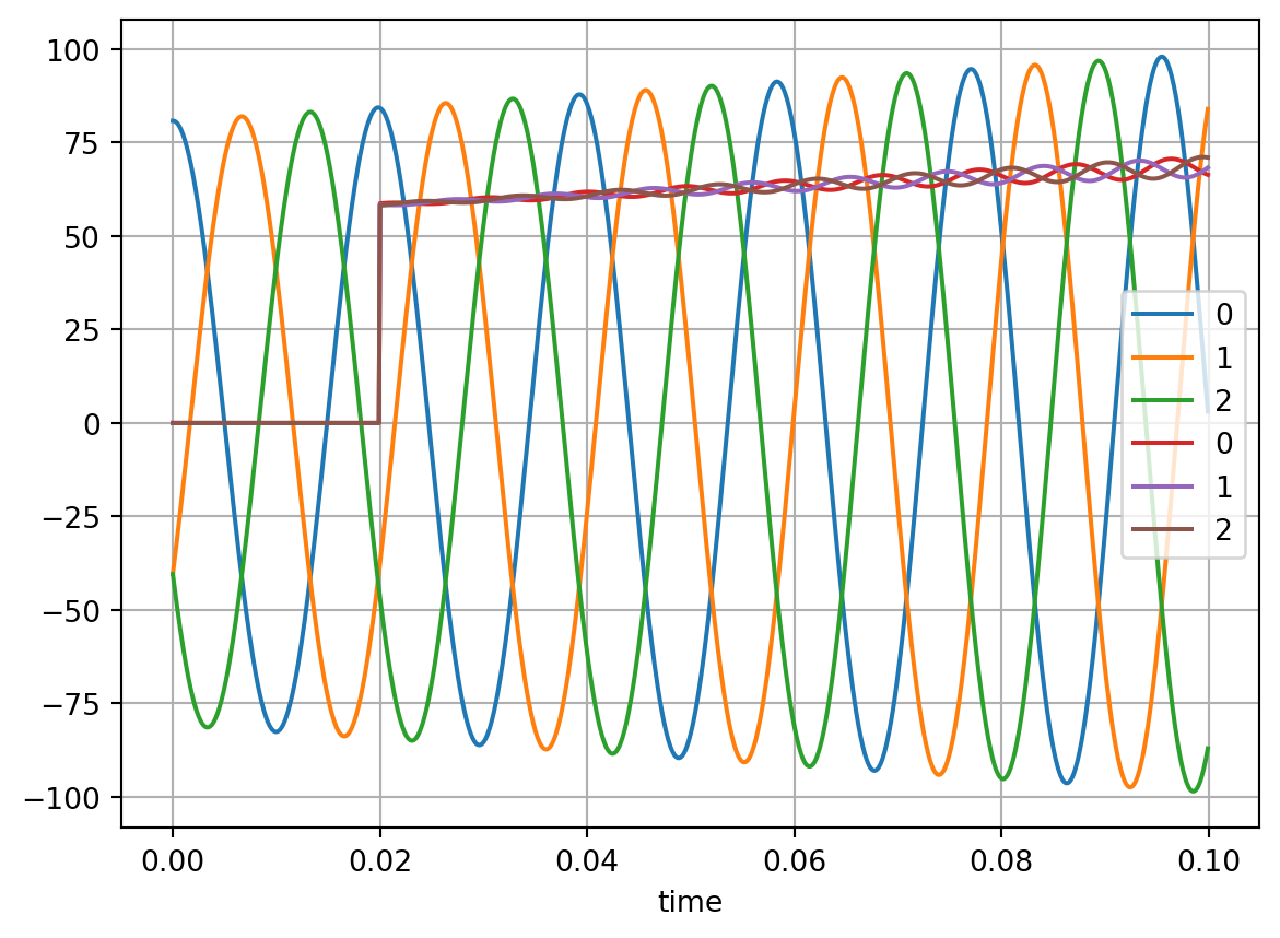
Currently, only a first-order low-pass filter (PT1) is implemented.
from trimes.filterimport pt1_filtercosine_wave_series_3_phase.plot(label="original")plt.title("Original Signal")filt = pt1_filter(cosine_wave_series_3_phase, 0.01, sample_time)filt.plot()plt.title("Filtered Signal (PT1)")
Text(0.5, 1.0, 'Filtered Signal (PT1)')
5 Fourier Analysis
A Fast Fourier Transform (FFT) implementation is planned for future releases.
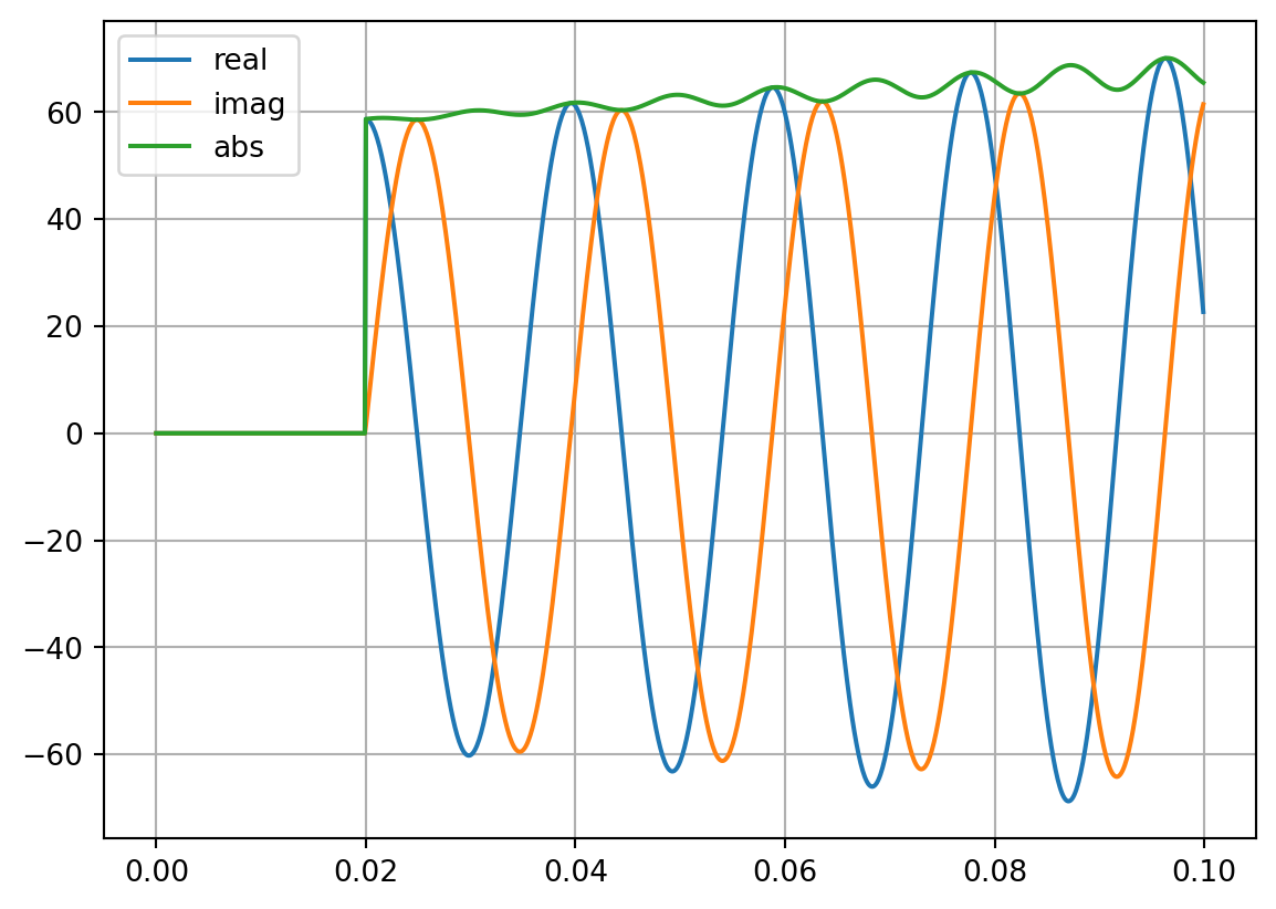
5.1 Fourier Coefficient
Fourier coefficients can be computed for a selected harmonic order (default: first harmonic).