Dynamic Modal Analysis

1 Introduction

Modal (small-signal) analysis linearizes the system around its current operating point and computes the eigenvalues of the resulting state matrix - one eigenvalue per oscillatory or non-oscillatory mode of the system. These eigenvalues describe the system’s small-signal stability: whether it returns to the operating point after a small enough disturbance that the linearization still holds - as opposed to large-signal (transient) stability, which asks the same question for one specific, possibly large, disturbance and can only be answered by a nonlinear time-domain simulation. A mode is stable exactly when its eigenvalue’s real part is negative.

Each eigenvalue \(\lambda = \sigma + j\omega\) is reported as two derived quantities that are easy to conflate: the decay rate \(\sigma\) (its real part, in 1/s - how fast the mode’s envelope decays, independent of how fast it oscillates) and the dimensionless damping ratio \(\zeta = -\sigma / |\lambda| = -\sigma / \sqrt{\sigma^2 + \omega^2}\). Unlike the decay rate, \(\zeta\) does depend on the imaginary part \(\omega\): two modes with the same decay rate but different oscillation frequencies have different damping ratios, since the faster-oscillating one completes - and therefore decays across - more cycles in the same time. A purely real eigenvalue has no oscillation to normalize by, so \(\zeta = 1\) by convention. Participation factors say which states (rotor angles, speeds, controller states, …) are involved in each mode.

This is complementary to a time-domain simulation: modal analysis tells you directly and exhaustively which modes exist and how well damped they are, without needing to pick a disturbance large enough (or simulate long enough) for a poorly-damped mode to become visible in a time trace - the last section of this tutorial compares the two directly.

powfacpy.applications.dynamic_modal_analysis wraps PowerFactory’s modal analysis command (ComMod) into ModalAnalysis (one eigen-decomposition of the current state) and ModalAnalysisResults (eigenvalues, damping ratios, frequencies, participation factors and eigenvectors, with filtering, plotting and eigenvalue tracking). A parameter sweep - how the eigenvalues move as something in the model changes - is not a separate sweep loop here: it is built on parstudy.Study, exactly like powfacpy.applications.parameter_studies - evaluate() calls ModalAnalysis.run() once per point, parstudy handles the sweep strategy and snapshot/restore, and track_eigenvalues() / EigenvalueSweepResults turn the resulting sequence of results into a consistently-indexed eigenvalue trajectory (PowerFactory does not guarantee eigenvalues come back in the same order run to run), with a root-locus plot and sensitivity helpers on top - two independent kinds of sensitivity, in fact: sensitivity_between finite-differences the eigenvalues between two tracked runs, while eigenvalue_sensitivity gets the same derivative analytically from the eigenvectors of a single run, with no tracking needed at all.

Needs the optional scipy dependency (pip install powfacpy[dynamic_modal_analysis]); the sweep and sensitivity helpers additionally need parstudy (pip install powfacpy[parstudy]).

2 Setup

First, we activate the PowerFactory project, i.e. the IEEE 39 bus system.

# If you use IPython/Jupyter:
import sys
import json

with open(r"..\..\settings_local.json") as settings_file:
    SETTINGS = json.load(settings_file)

sys.path.append(
    SETTINGS["local path to PowerFactory application"] # e.g. r"C:\Program Files\DIgSILENT\PowerFactory 2025 SP5\Python\3.13"
)
# Get the PF app
import powerfactory
import powfacpy

app = powerfactory.GetApplication()
app.Show()
app.ActivateProject(
    r"powfacpy\39_bus_new_england_copy_to_run_tests"
)  # You may change the project path.

0

We copy a study case with a valid, stable operating point - modal analysis only needs a valid operating point, not a disturbance - and then swap out its pre-configured events for a small load step. A short-circuit fault (used elsewhere in these tutorials) is a large disturbance - a discrete switching event, a voltage collapse near the fault, possibly protection tripping - that pushes the system well outside where a linearization is valid, whereas modal analysis’ own premise is precisely that the disturbance stays small; a modest load step keeps the time-domain comparison later in this tutorial honestly comparable to the linearized modal-analysis results. We also get the synchronous machines whose inertia we’ll be perturbing.

from powfacpy.base.active_project import ActiveProject
from powfacpy.applications.dynamic_simulation import DynamicSimulation

act_prj = ActiveProject(app)
act_prj.create_study_case(
    "Dynamic Modal Analysis", r"Study Cases\2.1 Simulation Fault Bus 16 Stable", parent_folder=r"Study Cases\powfacpy"
)
act_prj.clear_results_variables()
pfds = DynamicSimulation(app)

from powfacpy.result_variables import ResVar
RMS_BAL = ResVar.RMS_Bal

try:
    app.Hide()
    synchronous_machines = act_prj.get_calc_relevant_obj("ElmSym")
    synchronous_machines.sort(key=lambda x: x.loc_name)
    synchronous_machine_types = [sm.typ_id for sm in synchronous_machines]
    act_prj.add_results_variable(synchronous_machines, RMS_BAL.ElmSym.s_speed.value)

    # drop every event copied in with the study case (the fault, its clearance,
    # and an unrelated turbine-power event) and add a single, small load step
    loads = act_prj.get_calc_relevant_obj("ElmLod")
    loads.sort(key=lambda x: x.loc_name)
    load_step_target = loads[0]
    for event in app.GetFromStudyCase("IntEvt").GetContents("*.Evt*"):
        event.Delete()
    pfds.create_dyn_sim_event(
        "Load Step.EvtLod", {"p_target": load_step_target, "time": 1.0, "dP": 10.0}
    )
finally:
    app.Show()

3 A Single Modal Analysis

ModalAnalysis works on whatever state is currently active - like DynamicSimulation or StaticCalc. .run() executes PowerFactory’s modal analysis command and returns a ModalAnalysisResults:

from powfacpy.applications.dynamic_modal_analysis import ModalAnalysis

ma = ModalAnalysis(app)

try:
    app.Hide()
    results = ma.run()
finally:
    app.Show()

len(results)

166

get_dataframe() (or show() for a styled version) lists every eigenvalue with its real/imaginary part, damping ratio, natural/damped frequency, a "Mode" display string, and its dominant states (participation >= 5%):

results.get_dataframe().round(4).head(10)

	Real (1/s)	Imag (rad/s)	Undamped natural frequency (Hz)	Damped frequency (Hz)	Damping ratio	Mode	Dominant states
Index
1	-84.8959	0.0	0.0	0.0	1.0	-84.8959	Grid\G 04.ElmSym\psi1q,Grid\G 07.ElmSym\psi1q
2	-72.1759	0.0	0.0	0.0	1.0	-72.1759	Grid\G 02.ElmSym\psi1q,Grid\G 04.ElmSym\psi1q,...
3	-66.6192	0.0	0.0	0.0	1.0	-66.6192	Grid\G 02.ElmSym\psi1q
4	-49.7922	0.0	0.0	0.0	1.0	-49.7922	Grid\G 08.ElmSym\psi1q,Grid\G 10.ElmSym\psi1q
5	-48.2165	-0.0	0.0	0.0	1.0	-48.2165	Grid\Power Plant 07\AVR 07.ElmDsl\xa
6	-48.3471	-0.0	0.0	0.0	1.0	-48.3471	Grid\Power Plant 05\AVR 05.ElmDsl\xa
7	-49.1068	0.0	0.0	0.0	1.0	-49.1068	Grid\Power Plant 09\AVR 09.ElmDsl\xa
8	-49.3551	-0.0	0.0	0.0	1.0	-49.3551	Grid\Power Plant 06\AVR 06.ElmDsl\xa,Grid\Powe...
9	-49.3425	-0.0	0.0	0.0	1.0	-49.3425	Grid\Power Plant 06\AVR 06.ElmDsl\xa,Grid\Powe...
10	-44.1827	0.0	0.0	0.0	1.0	-44.1827	Grid\G 06.ElmSym\psi1q,Grid\G 08.ElmSym\psi1q,...

All ten of these happen to be real (zero imaginary part) - not a coincidence, but also not “the 10 most important eigenvalues”: get_dataframe() sorts by each eigenvalue’s index, i.e. its raw position in PowerFactory’s own state matrix (Amat.mtl), not by any measure of significance, so head(10) is just an arbitrary slice of all 166 eigenvalues. Their Dominant states above explain why these particular ones are real: single first-order states - a synchronous machine’s subtransient flux linkage (psi1q) or an exciter’s own internal lag state (xa, from avr_IEEET1) - decay directly, without oscillating, on their own. Oscillatory (complex-conjugate) eigenvalue pairs need two coupled states instead, such as a rotor angle together with its own speed - see the poorly-damped modes below, whose dominant states are exactly speed/phi pairs.

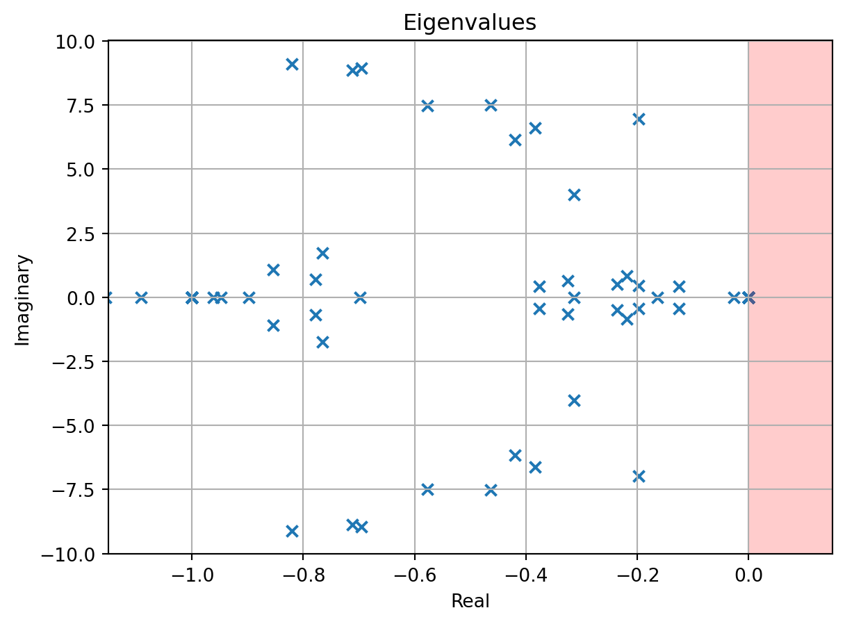
.plot() scatters the eigenvalues in the complex plane (the right half-plane, shaded, would be unstable - none are, here). By default (xlim="auto") the x-axis is zoomed to the dominant eigenvalues - those with the largest (least negative) real part, i.e. the slowest-decaying ones, which are what actually matters for how long a disturbance’s effect visibly persists - rather than the full range, which the fast, heavily-damped ones above (real parts around -45 to -85) would otherwise stretch until the dominant ones are an unreadable cluster near the origin. Concretely, the lower bound is the quantile-th percentile of all the real parts (quantile=0.75 by default, so roughly the most dominant quarter of eigenvalues stay in view); pass a higher quantile (closer to 1) to zoom in on fewer, even more dominant eigenvalues, a lower one to include more of the faster ones, or an explicit xlim=(lo, hi) to set the range directly (xlim=None restores matplotlib’s own full-range default):

results.plot();

3.1 Filtering

The poorly-damped modes are usually the interesting ones. Filtering methods return a new ModalAnalysisResults rather than mutating results, so they chain: filter_out_real_modes() keeps only the oscillatory eigenvalues, and filter_by_damping_ratio(...) then keeps those at or below a threshold:

poorly_damped = results.filter_out_real_modes().filter_by_damping_ratio(0.1)
poorly_damped.get_dataframe().round(4)

	Real (1/s)	Imag (rad/s)	Undamped natural frequency (Hz)	Damped frequency (Hz)	Damping ratio	Mode	Dominant states
Index
32	-0.8206	-9.1113	1.4560	1.4501	0.0897	-0.8206 ± 9.1113j	Grid\G 04.ElmSym\speed,Grid\G 04.ElmSym\phi,Gr...
33	-0.7117	-8.8591	1.4145	1.4100	0.0801	-0.7117 ± 8.8591j	Grid\G 08.ElmSym\speed,Grid\G 08.ElmSym\phi
34	-0.6961	-8.9388	1.4270	1.4226	0.0776	-0.6961 ± 8.9388j	Grid\G 06.ElmSym\speed,Grid\G 06.ElmSym\phi,Gr...
35	-0.8206	9.1113	1.4560	1.4501	0.0897	-0.8206 ± 9.1113j	Grid\G 04.ElmSym\speed,Grid\G 04.ElmSym\phi,Gr...
36	-0.7117	8.8591	1.4145	1.4100	0.0801	-0.7117 ± 8.8591j	Grid\G 08.ElmSym\speed,Grid\G 08.ElmSym\phi
37	-0.6961	8.9388	1.4270	1.4226	0.0776	-0.6961 ± 8.9388j	Grid\G 06.ElmSym\speed,Grid\G 06.ElmSym\phi,Gr...
38	-0.4635	-7.5107	1.1976	1.1954	0.0616	-0.4635 ± 7.5107j	Grid\G 02.ElmSym\speed,Grid\G 03.ElmSym\speed,...
39	-0.5766	-7.4771	1.1936	1.1900	0.0769	-0.5766 ± 7.4771j	Grid\G 04.ElmSym\speed,Grid\G 05.ElmSym\speed,...
40	-0.1971	-6.9749	1.1105	1.1101	0.0282	-0.1971 ± 6.9749j	Grid\G 10.ElmSym\speed,Grid\G 10.ElmSym\phi
41	-0.3834	-6.6123	1.0541	1.0524	0.0579	-0.3834 ± 6.6123j	Grid\G 01.ElmSym\phi,Grid\G 02.ElmSym\speed,Gr...
42	-0.4635	7.5107	1.1976	1.1954	0.0616	-0.4635 ± 7.5107j	Grid\G 02.ElmSym\speed,Grid\G 03.ElmSym\speed,...
43	-0.5766	7.4771	1.1936	1.1900	0.0769	-0.5766 ± 7.4771j	Grid\G 04.ElmSym\speed,Grid\G 05.ElmSym\speed,...
44	-0.1971	6.9749	1.1105	1.1101	0.0282	-0.1971 ± 6.9749j	Grid\G 10.ElmSym\speed,Grid\G 10.ElmSym\phi
45	-0.3834	6.6123	1.0541	1.0524	0.0579	-0.3834 ± 6.6123j	Grid\G 01.ElmSym\phi,Grid\G 02.ElmSym\speed,Gr...
46	-0.4194	-6.1521	0.9814	0.9791	0.0680	-0.4194 ± 6.1521j	Grid\G 09.ElmSym\speed,Grid\G 09.ElmSym\phi
47	-0.4194	6.1521	0.9814	0.9791	0.0680	-0.4194 ± 6.1521j	Grid\G 09.ElmSym\speed,Grid\G 09.ElmSym\phi
67	-0.3136	-4.0127	0.6406	0.6386	0.0779	-0.3136 ± 4.0127j	Grid\G 01.ElmSym\speed,Grid\G 01.ElmSym\phi,Gr...
68	-0.3136	4.0127	0.6406	0.6386	0.0779	-0.3136 ± 4.0127j	Grid\G 01.ElmSym\speed,Grid\G 01.ElmSym\phi,Gr...

3.2 Participation Factors

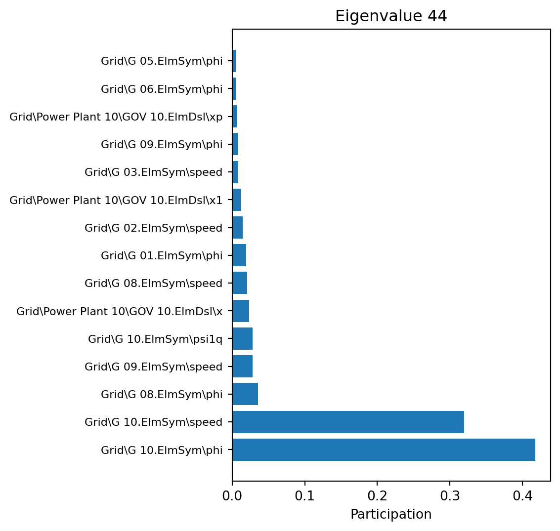
get_participation_dataframe() (or show_participation(), with a colour gradient) gives the full (state, eigenvalue) matrix; plot_participation() draws a bar chart per eigenvalue. filter_by_index(...) (an eigenvalue’s Index, from the table above) narrows down to one mode - here, the worst-damped oscillatory one:

worst_mode_index = poorly_damped.get_dataframe()["Damping ratio"].idxmin()
results.filter_by_index(worst_mode_index).plot_participation();

4 Sweeping a Parameter

How do the eigenvalues move as a parameter changes? As in the Parameter Studies tutorial, we declare the swept quantity as a parstudy.ModelParameter and give a Study an evaluate function - here, evaluate just runs the modal analysis and returns a couple of scalar metrics (for the results table) alongside the full ModalAnalysisResults (as raw, for the eigenvalue trajectory below). We sweep every machine’s inertia together, ±50% around its own value:

from parstudy import ModelParameter, linspace, Study

h_param = ModelParameter(
    "H (multiply)", linspace(0.5, 1.5, 5),
    affects=[(t, "tag") for t in synchronous_machine_types],
    mode="multiply",
)

def evaluate(values):
    modal_results = ma.run()
    worst = modal_results.filter_out_real_modes().get_dataframe()["Damping ratio"]
    return {
        "worst_damping_ratio": float(worst.min()),
    }, modal_results

try:
    app.Hide()
    sweep_results = Study([h_param], evaluate).run(verbose=1)
finally:
    app.Show()

sweep_results.evaluations.iloc[1:,:].round(4)

[1/6] sample
[2/6] H (multiply)=0.5
[3/6] H (multiply)=0.75
[4/6] H (multiply)=1.0
[5/6] H (multiply)=1.25
[6/6] H (multiply)=1.5

	parameters	results
	H (multiply)	worst_damping_ratio
run
1	0.50	0.0534
2	0.75	0.0369
3	1.00	0.0282
4	1.25	0.0233
5	1.50	0.0204

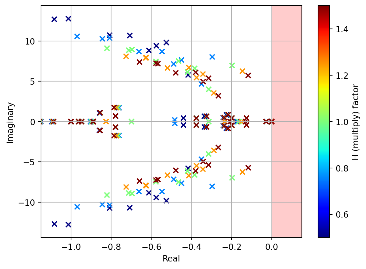
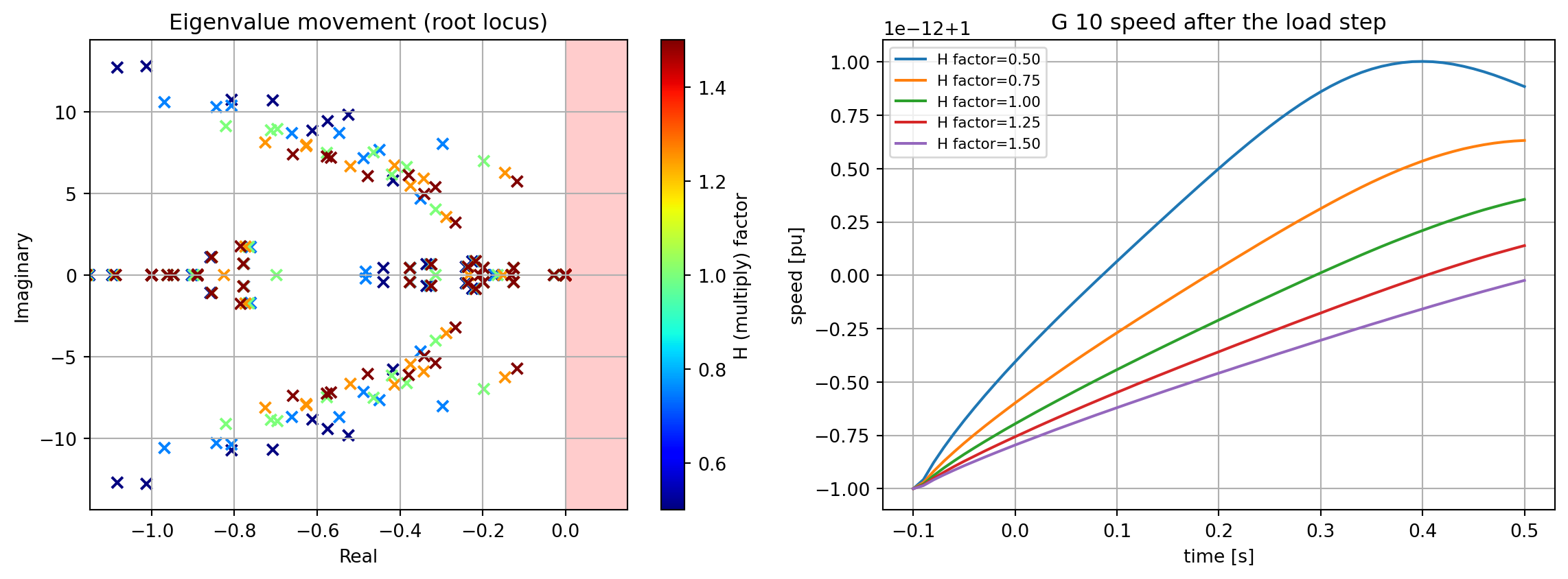
Scaling every machine’s inertia down (H (multiply) < 1) raises every mode’s frequency and, here, also its damping ratio; scaling it up does the opposite - inertia and the electromechanical modes’ frequency are directly linked. (worst_damping_ratio is simply whichever mode is worst-damped in each individual run here - not necessarily the same physical mode throughout; the next section tracks the eigenvalues properly.)

4.1 Tracking Eigenvalues Across the Sweep

PowerFactory does not guarantee the eigenvalues come back in the same order from run to run, so comparing them index-by-index across runs would risk comparing unrelated modes. EigenvalueSweepResults.from_study_results(sweep_results, parameter_name) pulls the swept parameter’s value and each run’s raw ModalAnalysisResults out of the parstudy.StudyResults; .track_eigenvalues() then reorders every run’s eigenvalues to match the previous run’s, so eigenvalue index k refers to the same physical mode throughout the sweep:

from powfacpy.applications.dynamic_modal_analysis import EigenvalueSweepResults

sweep = EigenvalueSweepResults.from_study_results(sweep_results, "H (multiply)").track_eigenvalues()
len(sweep)

6

.plot() is the classic root locus view: every run’s eigenvalues, coloured by the parameter value, with the same xlim/quantile auto-zoom to the dominant eigenvalues as above (computed here across every run in the sweep):

sweep.plot(colorbar_label="H (multiply) factor");

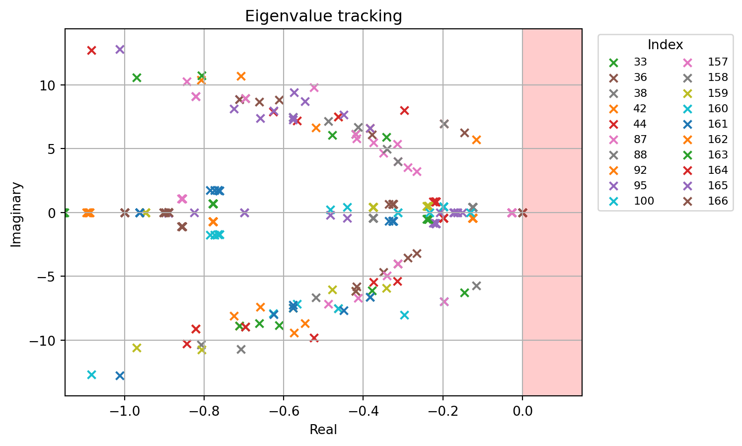
.plot_eigenvalue_tracking() colours and labels by eigenvalue index instead of by parameter value - a sanity check that tracking followed each mode continuously rather than jumping between modes (a mode that appears to teleport between two very different positions from one point to the next signals a tracking mistake, e.g. too large a step between swept values):

sweep.plot_eigenvalue_tracking();

5 Modal Sensitivity

sensitivity_between(before, after) tracks after’s eigenvalues against before’s and returns the per-eigenvalue change in every metric - a quick before/after comparison without plotting the whole sweep. Comparing the two extremes already computed above:

from powfacpy.applications.dynamic_modal_analysis import sensitivity_between

sensitivity = sensitivity_between(sweep.when_index(0), sweep.when_index(-1))
sensitivity.filter_out_real_modes().filter_by_metrics(["Damping ratio", "Damped frequency (Hz)"]).show()

	Damping ratio	Damped frequency (Hz)
Index
25	0.0001	0.0002
26	0.0001	0.0002
32	-0.0211	-0.6607
33	-0.0597	-0.4987
34	-0.0193	-0.5668
35	-0.0211	-0.6607
36	-0.0597	-0.4987
37	-0.0193	-0.5668
38	0.0176	-0.0408
39	0.0119	-0.0145
40	0.0504	0.0330
41	0.0208	-0.0892
42	0.0176	-0.0408
43	0.0119	-0.0145
44	0.0504	0.0330
45	0.0208	-0.0892
46	-0.0062	-0.0061
47	-0.0062	-0.0061
64	-0.0000	0.0000
65	-0.0000	0.0000
67	0.0046	-0.1280
68	0.0046	-0.1280
71	0.0001	-0.0020
72	0.0001	-0.0020
80	0.0024	0.0050
81	0.0024	0.0050
84	-0.0026	0.0003
85	-0.0026	0.0003
86	-0.0007	-0.0002
88	-0.0007	0.0000
89	-0.0017	0.0000
90	-0.0006	0.0001
91	-0.0007	-0.0002
92	-0.0007	0.0000
93	-0.0017	0.0000
94	-0.0006	0.0001
96	-0.0020	0.0010
97	-0.0020	0.0010
98	0.0002	0.0001
99	0.0002	0.0001
102	-0.0008	0.0004
103	-0.0008	0.0004
108	0.0023	-0.0050
110	0.0023	-0.0050
114	0.0000	-0.0001
115	0.0001	-0.0002
116	0.0001	-0.0002
117	0.0000	-0.0002
119	0.0000	-0.0001
120	-0.0000	0.0002
121	-0.0000	0.0002
122	0.0001	-0.0002
123	0.0000	-0.0002
124	0.0001	-0.0002
128	0.0000	-0.0000
129	0.0000	-0.0000
130	0.0000	-0.0001
131	0.0000	-0.0000
134	0.0000	-0.0001
135	0.0000	-0.0000

5.1 Parametric Sensitivity

To see how a sensitivity itself depends on a second, condition quantity, sweep both together and slice the (tracked) results by condition afterwards. Below, the condition is which single machine type’s inertia gets perturbed (±20% this time) - a direct way to ask “which generator’s inertia does a given mode’s damping actually care about?” condition isn’t itself a PF attribute, so it is a plain (auto_apply=False) ModelParameter whose values are the machine-type objects themselves, and evaluate applies the perturbation to whichever one context says is active this run:

from powfacpy.applications.dynamic_modal_analysis import track_eigenvalues, ParametricSensitivity

condition_types = synchronous_machine_types[:3]
h_baseline = {t: t.GetAttribute("tag") for t in condition_types}

condition_param = ModelParameter("condition", condition_types, auto_apply=False)
h_2point = ModelParameter("H", [0.8, 1.2], auto_apply=False)

def evaluate_2d(values, context):
    typ = values["condition"]
    typ.SetAttribute("tag", h_baseline[typ] * values["H"])
    modal_results = ma.run()
    typ.SetAttribute("tag", h_baseline[typ])  # auto_apply=False -> restore ourselves
    return {}, modal_results

try:
    app.Hide()
    results_2d = Study([condition_param, h_2point], evaluate_2d, strategy="grid").run(verbose=1)
finally:
    app.Show()

[1/6] sample
[2/6] sample
[3/6] sample
[4/6] sample
[5/6] sample
[6/6] sample

strategy="grid" visits every (condition, H) combination - 3 conditions x 2 values of H here, with no baseline row, which is exactly the pair of points each sensitivity needs. We track all six runs in one continuous sequence (not condition by condition) so that eigenvalue index k keeps meaning the same physical mode across every condition, then split the tracked sequence back into three (before, after) pairs - one per condition, in the same order results_2d visited them:

all_tracked = track_eigenvalues([results_2d.raw(r.index) for r in results_2d.records])

sensitivities = [
    sensitivity_between(all_tracked[i], all_tracked[i + 1])
    for i in range(0, len(all_tracked), 2)
]
parametric_sensitivity = ParametricSensitivity(
    [t.loc_name for t in condition_types], sensitivities
)
(
    parametric_sensitivity.filter_out_real_modes()
    .filter_by_damping_ratio(0.2)
    .filter_by_metrics("Damping ratio")
    .normalize("column")
    .show()
)

	Type Gen 01	Type Gen 02	Type Gen 03
Index
32	-0.0255	0.0735	1.0000
33	-0.0255	0.0735	1.0000
34	-0.0246	0.0789	1.0000
35	1.0000	-0.1864	-6.5312
37	-0.0246	0.0789	1.0000
38	1.0000	-0.1864	-6.5312
39	0.0010	-1.9258	1.0000
40	1.0000	283.0773	189.7602
41	1.0000	-26.9132	-15.2880
42	-0.0168	1.0000	0.2163
43	1.0000	-29.2984	-13.8492
44	0.0010	-1.9258	1.0000
45	1.0000	283.0773	189.7602
46	1.0000	-26.9132	-15.2880
47	-0.0168	1.0000	0.2163
48	1.0000	-29.2984	-13.8492
65	1.0000	-0.0203	-0.0142
66	1.0000	-0.0203	-0.0142

Reading a row: for that mode, the darkest cell names the machine type whose inertia its damping ratio is most sensitive to - typically not all three alike, since each mode is dominated by a different subset of machines (recall the participation factors above).

6 Eigenvalue Sensitivity: Analytical vs. Finite-Difference

sensitivity_between above finite-differences the eigenvalues themselves between two (tracked) runs. There is a second, classical way to get the same derivative that needs no eigenvalue tracking at all: the eigenvector-weighted sensitivity formula [1, 2]

\[\frac{d\lambda_i}{dp} \approx \frac{\psi_i^H \,(dA/dp)\, \phi_i}{\psi_i^H \phi_i}\]

where \(\phi_i\)/\(\psi_i\) are the right/left eigenvectors of mode \(i\) - ModalAnalysis.run() already computes them (they’re what the participation factors above are built from), and ModalAnalysisResults keeps them (get_right_eigenvectors()/get_left_eigenvectors()). Since it only uses one run’s eigenvectors, it sidesteps eigenvalue tracking entirely - handy when two modes are close enough that tracking could plausibly mix them up. dA/dp is usually itself a finite difference of the state matrix between two runs (system_matrix_sensitivity), not of the eigenvalues - so both approaches still need two modal analyses, they just finite-difference a different quantity.

This time we perturb a real controller parameter - Ka, the gain of generator G 05’s automatic voltage regulator (an IEEE Type 1 exciter, avr_IEEET1) - by a small amount:

avr = act_prj.get_unique_obj(r"Network Model\Network Data\Grid\Power Plant 05\AVR 05")
baseline_params = list(avr.GetAttribute("params"))
Ka_index = 1  # avr_IEEET1's parameter order: Tr,Ka,Ta,Ke,Te,Kf,Tf,E1,Se1,E2,Se2

delta = 0.1
perturbed_params = list(baseline_params)
perturbed_params[Ka_index] += delta

try:
    app.Hide()
    before = ma.run()
    avr.SetAttribute("params", perturbed_params)
    after = ma.run()
finally:
    avr.SetAttribute("params", baseline_params)
    app.Show()

system_matrix_sensitivity(before, after, delta) gives a finite-difference estimate of dA/dKa; before.eigenvalue_sensitivity(mode_index, delta_matrix) then applies the formula above using before’s own eigenvectors - no tracking involved. We compare it against sensitivity_between(before, after) (divided by delta, the same finite-difference-on-eigenvalues approach as above) for every mode dominated by this AVR’s own states:

import pandas as pd
from powfacpy.applications.dynamic_modal_analysis import system_matrix_sensitivity

delta_A = system_matrix_sensitivity(before, after, delta)
finite_difference = sensitivity_between(before, after).get_dataframe() / delta

avr_modes = before.get_dataframe()
avr_modes = avr_modes[avr_modes["Dominant states"].str.contains("AVR 05")]

pd.DataFrame(
    {
        "analytical (eigenvectors)": [
            before.eigenvalue_sensitivity(idx, delta_A) for idx in avr_modes.index
        ],
        "finite difference (eigenvalues)": [
            complex(finite_difference.loc[idx, "Real (1/s)"], finite_difference.loc[idx, "Imag (rad/s)"])
            for idx in avr_modes.index
        ],
    },
    index=avr_modes.index,
).round(5)

	analytical (eigenvectors)	finite difference (eigenvalues)
Index
6	0.04291-0.00000j	0.04292+0.00000j
96	-0.00646-0.00391j	-0.00646-0.00390j
97	-0.00646+0.00391j	-0.00646+0.00390j
101	-0.02832-0.00000j	-0.02833+0.00000j
102	-0.00078-0.00032j	-0.00078-0.00032j
103	-0.00078+0.00032j	-0.00078+0.00032j
160	0.00000+0.00000j	0.00000+0.00000j

The two independent approaches agree to 4-5 decimal places for every mode - a useful cross-check when eigenvalue tracking is in doubt (two nearby modes, a large step between runs, …). The fastest of the group (real part around -48, dominated by the AVR’s own state xa) is by far the most sensitive to Ka, as expected for a gain acting directly on that state; the electromechanical modes further up the table are only weakly affected, since Ka mainly shapes the AVR’s own fast dynamics.

7 Connecting Modal Analysis to a Time-Domain Simulation

Modal analysis and a time-domain simulation describe the same system from two angles: modal analysis linearizes around the operating point and reports every mode’s frequency and damping directly and exhaustively; a simulation shows the full response to one actual disturbance, which - for a small enough disturbance that the linearization still applies - is approximately the superposition of all those modes. The same parameter sweep should therefore tell a consistent story in both, provided the disturbance is one the linearization can actually speak to; that is why this section reuses the small load step from the setup above rather than a large fault. evaluate below runs the modal analysis first (at the pre-disturbance operating point) and then the load-step simulation already set up in this study case, storing both:

from powfacpy.applications.results import Results

pfri = Results(app)
pfri.pf_objects_in_labels = True

h_param_small = ModelParameter(
    "H (multiply)", linspace(0.5, 1.5, 5),
    affects=[(t, "tag") for t in synchronous_machine_types],
    mode="multiply",
)

sim_traces = []

def evaluate_with_sim(values):
    modal_results = ma.run()
    worst = modal_results.filter_out_real_modes().get_dataframe()

    pfds.initialize_and_run_sim()
    sim_res = pfri.export_to_pandas()
    sim_traces.append(sim_res)

    return {
        "worst_damping_ratio": float(worst["Damping ratio"].min()),
        "worst_damped_freq_Hz": float(worst.loc[worst["Damping ratio"].idxmin(), "Damped frequency (Hz)"]),
    }, modal_results

try:
    app.Hide()
    combined_results = Study([h_param_small], evaluate_with_sim).run(verbose=1)
finally:
    app.Show()

combined_results.evaluations.round(4)

[1/6] sample

C:\Users\seberlein\local\FraunhIEE-UniKassel-PowSysStability\powfacpy\src\powfacpy\base\active_project.py:249: UserWarning: The returned *.ElmRes object is not unique in the  study case: 'Study Cases\powfacpy\Dynamic Modal Analysis'. Make sure that the correct *.ElmRes object is used: <l3>\seberlein.IntUser\powfacpy\39_bus_new_england_copy_to_run_tests.IntPrj\Study Cases.IntPrjfolder\powfacpy\Dynamic Modal Analysis.IntCase\All calculations.ElmRes</l3>.
  warn(

[2/6] H (multiply)=0.5

C:\Users\seberlein\local\FraunhIEE-UniKassel-PowSysStability\powfacpy\src\powfacpy\base\active_project.py:249: UserWarning: The returned *.ElmRes object is not unique in the  study case: 'Study Cases\powfacpy\Dynamic Modal Analysis'. Make sure that the correct *.ElmRes object is used: <l3>\seberlein.IntUser\powfacpy\39_bus_new_england_copy_to_run_tests.IntPrj\Study Cases.IntPrjfolder\powfacpy\Dynamic Modal Analysis.IntCase\All calculations.ElmRes</l3>.
  warn(

[3/6] H (multiply)=0.75

C:\Users\seberlein\local\FraunhIEE-UniKassel-PowSysStability\powfacpy\src\powfacpy\base\active_project.py:249: UserWarning: The returned *.ElmRes object is not unique in the  study case: 'Study Cases\powfacpy\Dynamic Modal Analysis'. Make sure that the correct *.ElmRes object is used: <l3>\seberlein.IntUser\powfacpy\39_bus_new_england_copy_to_run_tests.IntPrj\Study Cases.IntPrjfolder\powfacpy\Dynamic Modal Analysis.IntCase\All calculations.ElmRes</l3>.
  warn(

[4/6] H (multiply)=1.0

C:\Users\seberlein\local\FraunhIEE-UniKassel-PowSysStability\powfacpy\src\powfacpy\base\active_project.py:249: UserWarning: The returned *.ElmRes object is not unique in the  study case: 'Study Cases\powfacpy\Dynamic Modal Analysis'. Make sure that the correct *.ElmRes object is used: <l3>\seberlein.IntUser\powfacpy\39_bus_new_england_copy_to_run_tests.IntPrj\Study Cases.IntPrjfolder\powfacpy\Dynamic Modal Analysis.IntCase\All calculations.ElmRes</l3>.
  warn(

[5/6] H (multiply)=1.25

C:\Users\seberlein\local\FraunhIEE-UniKassel-PowSysStability\powfacpy\src\powfacpy\base\active_project.py:249: UserWarning: The returned *.ElmRes object is not unique in the  study case: 'Study Cases\powfacpy\Dynamic Modal Analysis'. Make sure that the correct *.ElmRes object is used: <l3>\seberlein.IntUser\powfacpy\39_bus_new_england_copy_to_run_tests.IntPrj\Study Cases.IntPrjfolder\powfacpy\Dynamic Modal Analysis.IntCase\All calculations.ElmRes</l3>.
  warn(

[6/6] H (multiply)=1.5

C:\Users\seberlein\local\FraunhIEE-UniKassel-PowSysStability\powfacpy\src\powfacpy\base\active_project.py:249: UserWarning: The returned *.ElmRes object is not unique in the  study case: 'Study Cases\powfacpy\Dynamic Modal Analysis'. Make sure that the correct *.ElmRes object is used: <l3>\seberlein.IntUser\powfacpy\39_bus_new_england_copy_to_run_tests.IntPrj\Study Cases.IntPrjfolder\powfacpy\Dynamic Modal Analysis.IntCase\All calculations.ElmRes</l3>.
  warn(

	parameters	results
	H (multiply)	worst_damped_freq_Hz	worst_damping_ratio
run
0	1.00	1.1101	0.0282
1	0.50	1.5616	0.0534
2	0.75	1.2777	0.0369
3	1.00	1.1101	0.0282
4	1.25	0.9958	0.0233
5	1.50	0.9113	0.0204

Side by side: the root-locus view from modal analysis, and the actual simulated speed of one machine (G 10, dominant in one of the poorly-damped modes above) for every H in the same sweep. Lower inertia visibly pushes the eigenvalues up the imaginary axis (faster oscillation, matching worst_damped_freq_Hz above) and produces a visibly faster, larger swing in the simulated response - modal analysis and the time-domain simulation agree on the direction of the effect, as they must, since they describe the same system:

import matplotlib.pyplot as plt

# the baseline run (H factor=1.0) duplicates one of the swept values here, so
# we drop it from this plot with include_baseline=False.
combined_sweep = EigenvalueSweepResults.from_study_results(
    combined_results, "H (multiply)", include_baseline=False
).track_eigenvalues()

swept = [r.varied is not None for r in combined_results.records]
h_values = [
    h for h, keep in zip(combined_results.evaluations[("parameters", "H (multiply)")], swept) if keep
]
swept_traces = [sim_res for sim_res, keep in zip(sim_traces, swept) if keep]

fig, axes = plt.subplots(1, 2, figsize=(12, 4.5))

combined_sweep.plot(colorbar_label="H (multiply) factor", ax=axes[0])
axes[0].set_title("Eigenvalue movement (root locus)")

axes[1].set_title("G 10 speed after the load step")
g10 = [m for m in synchronous_machines if m.loc_name == "G 10"]
for h, sim_res in zip(h_values, swept_traces):
    speed = pfri.get_simulation_results_from_dataframe(sim_res, g10, RMS_BAL.ElmSym.s_speed.value).iloc[:, 0]
    axes[1].plot(speed.index, speed.to_numpy(), label=f"H factor={h:.2f}")
axes[1].set_xlabel("time [s]"); axes[1].set_ylabel("speed [pu]")
axes[1].legend(fontsize=8); axes[1].grid(True)
fig.tight_layout()

8 Where To Go From Here

• ModalAnalysis.run(commod_params={...}) passes additional/overriding ComMod parameters straight through (e.g. a different initMode, or a subset of eigenvalues via the isRec* filters) - see PowerFactory’s own documentation of ComMod for what’s available.
• Everything here composes with the rest of parstudy: a full grid, latin_hypercube(n) or sobol(n) sample is one strategy= argument to Study, and EigenvalueSweepResults.from_study_results works the same way regardless of the strategy used to produce sweep_results.
• ModalAnalysisResults.get_system_matrix() / .get_states() give the raw state matrix and state names; get_right_eigenvectors() / get_left_eigenvectors() give the raw eigenvectors behind the participation factors and eigenvalue_sensitivity - if you need something this module doesn’t already compute from them.
• Combine this with the Study Cases tutorial to keep a persistent, browsable study case for each point of a sweep you want to revisit by hand, rather than (or alongside) the in-memory parstudy sweep used here - see the Relation to the Study Cases tutorial note in the Parameter Studies tutorial.

References

[1]

J. I. Pérez-Arriaga, G. C. Verghese, and F. C. Schweppe, “Selective modal analysis with applications to electric power systems, Part I: Heuristic introduction,” IEEE Transactions on Power Apparatus and Systems, vol. PAS–101, no. 9, pp. 3117–3125, Sept. 1982, doi: 10.1109/TPAS.1982.317524.

[2]

G. C. Verghese, J. I. Pérez-Arriaga, and F. C. Schweppe, “Selective modal analysis with applications to electric power systems, Part II: The dynamic stability problem,” IEEE Transactions on Power Apparatus and Systems, vol. PAS–101, no. 9, pp. 3126–3134, Sept. 1982, doi: 10.1109/TPAS.1982.317525.